Evaluation Climate Variability (ERA5) CMIP6
CMIP6 Multi-Model Mean Context
Comparison with CMIP6 ensemble mean from 11 members.
Contributing models: ACCESS-ESM1-5, AWI-CM-1-1-MR, CNRM-CM6-1, CNRM-ESM2-1, EC-Earth3, FGOALS-g3, GISS-E2-1-G, INM-CM5-0, IPSL-CM6A-LR, MPI-ESM1-2-LR, MRI-ESM2-0
Synthesis
Related diagnostics
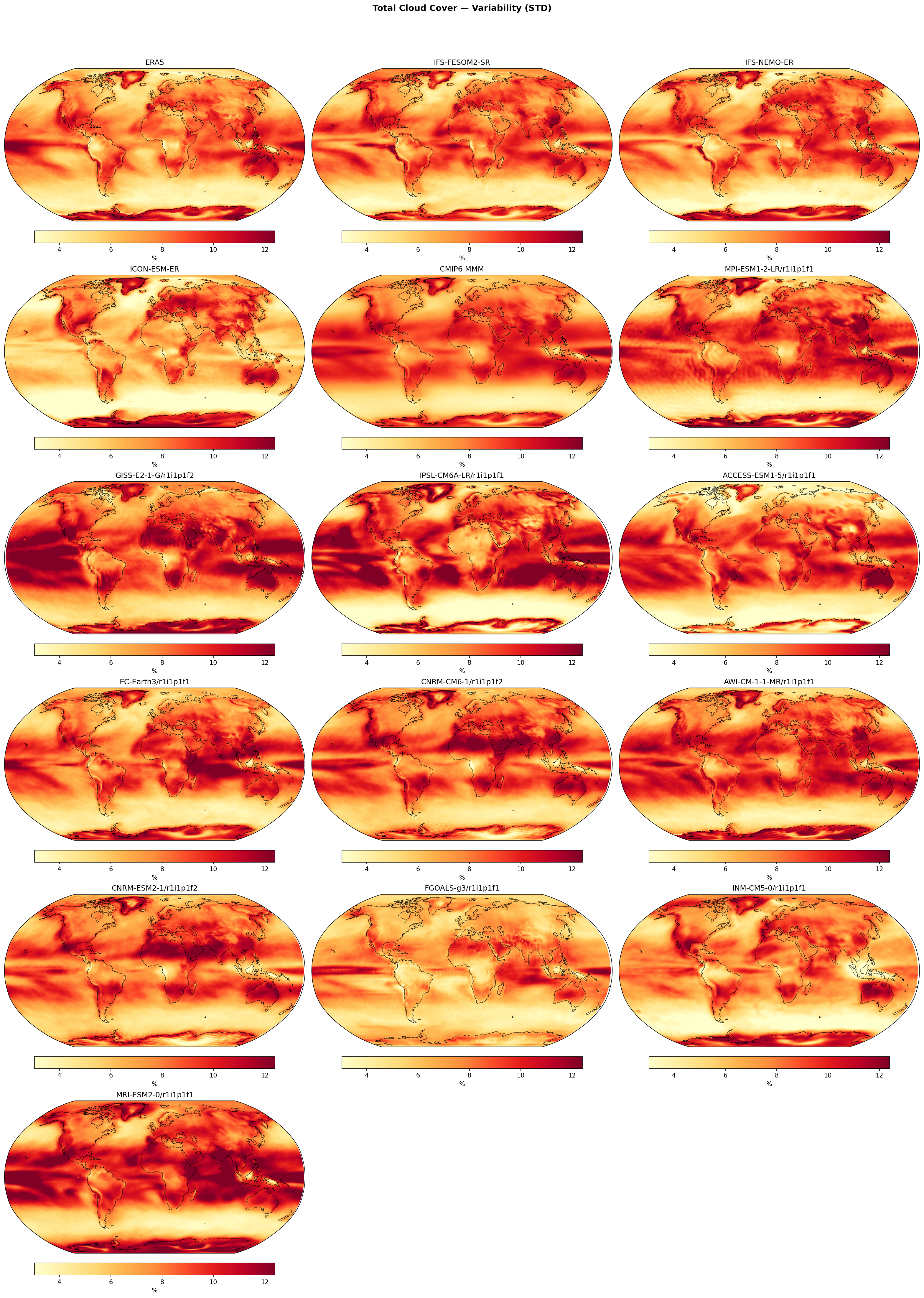
Total Cloud Cover — Variability (STD)
| Variables | clt |
|---|---|
| Models | IFS-FESOM2-SR, IFS-NEMO-ER, ICON-ESM-ER, CMIP6 MMM, MPI-ESM1-2-LR/r1i1p1f1, GISS-E2-1-G/r1i1p1f2, IPSL-CM6A-LR/r1i1p1f1, ACCESS-ESM1-5/r1i1p1f1, EC-Earth3/r1i1p1f1, CNRM-CM6-1/r1i1p1f2, AWI-CM-1-1-MR/r1i1p1f1, CNRM-ESM2-1/r1i1p1f2, FGOALS-g3/r1i1p1f1, INM-CM5-0/r1i1p1f1, MRI-ESM2-0/r1i1p1f1 |
| Reference Dataset | ERA5 |
| Units | % |
| Period | 1980–2014 |
| IFS-FESOM2-SR | Std Gmean: 7.59 · Diff Gmean: 0.24 · Rmse: 1.21 |
| IFS-NEMO-ER | Std Gmean: 7.39 · Diff Gmean: 0.04 · Rmse: 1.00 |
| ICON-ESM-ER | Std Gmean: 6.38 · Diff Gmean: -0.96 · Rmse: 2.03 |
| CMIP6 MMM | Std Gmean: 8.13 · Diff Gmean: 0.78 · Rmse: 1.28 |
Summary high
This diagnostic evaluates the temporal variability (standard deviation) of deseasonalised total cloud cover anomalies. The IFS-based high-resolution models closely replicate ERA5 variability patterns and magnitudes, whereas ICON-ESM-ER systematically underestimates cloud variability.
Key Findings
- IFS-NEMO-ER shows exceptional agreement with ERA5 (RMSE ~1.0%), accurately capturing high variability zones in the ITCZ and mid-latitude storm tracks.
- ICON-ESM-ER exhibits a global dampening of cloud variability (mean bias -0.96%), with notably weaker variance in the Southern Ocean and tropical Pacific compared to ERA5 and IFS models.
- The CMIP6 Multi-Model Mean generally overestimates variability (+0.78%), obscuring a wide spread among individual models—ranging from excessive variability in GISS-E2-1-G to suppressed variability in FGOALS-g3.
Spatial Patterns
High variability (>10%) is concentrated in the ENSO-dominated tropical Pacific and the North Atlantic/Pacific storm tracks. Low variability (<4%) characterizes the stable subtropical subsidence zones and desert regions. The IFS models successfully reproduce the sharp spatial gradients of variability seen in ERA5, particularly the 'wedge' shape in the central Pacific.
Model Agreement
There is strong agreement between the two IFS variants (FESOM2-SR and NEMO-ER) and ERA5. ICON-ESM-ER diverges from the high-resolution group, aligning more closely with low-variance CMIP6 models like FGOALS-g3 and INM-CM5-0.
Physical Interpretation
Cloud cover variability in these maps reflects the intensity of synoptic systems (storm tracks) and large-scale climate modes (e.g., ENSO in the Pacific). The realistic variability in IFS suggests its convection and cloud schemes respond appropriately to dynamical forcing. ICON's underestimation suggests a model tuning that favors persistence or overly stable cloud decks, damping the response to atmospheric disturbances.
Caveats
- ERA5 cloud cover is a reanalysis product (model-generated based on assimilation), not direct satellite observation, and carries its own uncertainties.
- The analysis uses monthly data, filtering out high-frequency synoptic variability (daily timescales).
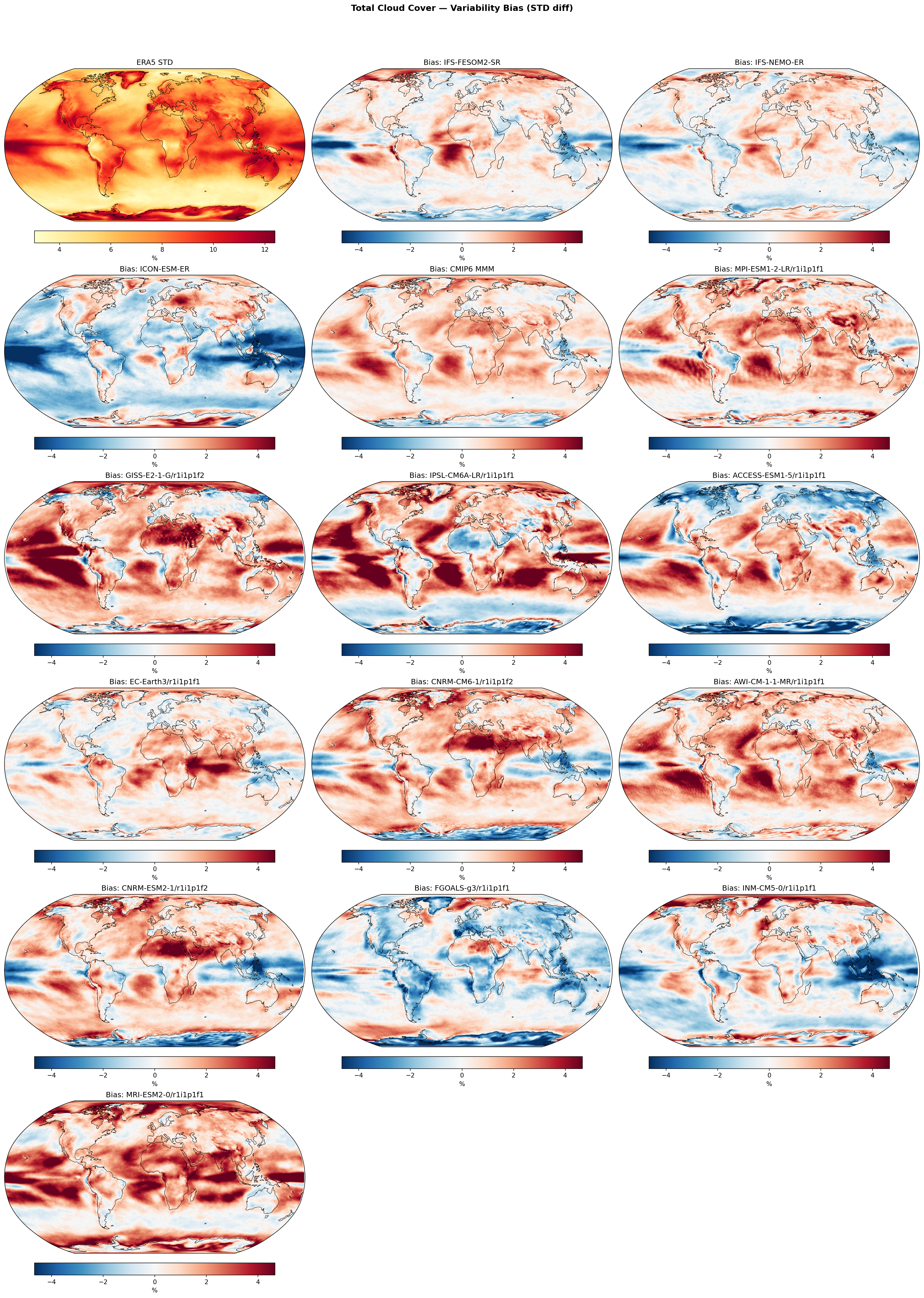
Total Cloud Cover — Variability Bias (STD diff)
| Variables | clt |
|---|---|
| Models | IFS-FESOM2-SR, IFS-NEMO-ER, ICON-ESM-ER, CMIP6 MMM, MPI-ESM1-2-LR/r1i1p1f1, GISS-E2-1-G/r1i1p1f2, IPSL-CM6A-LR/r1i1p1f1, ACCESS-ESM1-5/r1i1p1f1, EC-Earth3/r1i1p1f1, CNRM-CM6-1/r1i1p1f2, AWI-CM-1-1-MR/r1i1p1f1, CNRM-ESM2-1/r1i1p1f2, FGOALS-g3/r1i1p1f1, INM-CM5-0/r1i1p1f1, MRI-ESM2-0/r1i1p1f1 |
| Reference Dataset | ERA5 |
| Units | % |
| Period | 1980–2014 |
| IFS-FESOM2-SR | Std Gmean: 7.59 · Diff Gmean: 0.24 · Rmse: 1.21 |
| IFS-NEMO-ER | Std Gmean: 7.39 · Diff Gmean: 0.04 · Rmse: 1.00 |
| ICON-ESM-ER | Std Gmean: 6.38 · Diff Gmean: -0.96 · Rmse: 2.03 |
| CMIP6 MMM | Std Gmean: 8.13 · Diff Gmean: 0.78 · Rmse: 1.28 |
Summary high
This diagnostic evaluates the variability (standard deviation of monthly anomalies) of Total Cloud Cover compared to ERA5. The IFS-NEMO-ER model demonstrates the best agreement with observations, while ICON-ESM-ER significantly underestimates variability globally, and CMIP6 models generally overestimate it.
Key Findings
- IFS-NEMO-ER exhibits the lowest RMSE (1.00%) and a near-zero global mean bias (+0.04%), indicating excellent capture of cloud variability magnitude.
- ICON-ESM-ER shows a systematic negative bias (global mean -0.96%), indicating it underestimates month-to-month cloud cover variability across most ocean basins.
- CMIP6 models (MMM and individuals like IPSL-CM6A-LR, GISS-E2-1-G) tend to overestimate cloud variability (positive bias), particularly over the Southern Ocean, land masses, and Northern Hemisphere storm tracks.
- Both IFS variants and ICON show a negative variability bias along the tropical ITCZ, suggesting suppressed intraseasonal variability relative to ERA5 in convective regions.
Spatial Patterns
ERA5 shows high cloud variability (>10%) in the ITCZ and storm tracks. The high-resolution IFS models capture the extratropical patterns well but slightly underestimate variability in the deep tropics (blue bands along the equator). ICON-ESM-ER is distinctively 'blue' (low variability) across the global ocean. In contrast, many CMIP6 models (e.g., MRI-ESM2-0, AWI-CM-1-1-MR) display strong 'red' biases (excessive variability) over the Southern Ocean and continental interiors.
Model Agreement
IFS-NEMO-ER performs significantly better than the other high-resolution model (ICON) and the CMIP6 ensemble. There is large spread among individual CMIP6 models, with some (INM-CM5-0, FGOALS-g3) resembling ICON's low variability, while others (GISS, IPSL) show excessive variability.
Physical Interpretation
The underestimation of variability in the tropics by the high-res models may relate to the representation of organized convection and intraseasonal oscillations (like the MJO); if these are too regular or weak, monthly variance drops. The excessive variability in CMIP6 models over storm tracks suggests potential issues with the stability of cloud decks or overly sensitive cloud-circulation feedbacks. ICON's global dampening of variability suggests its cloud parameterizations might be too insensitive to dynamical perturbations.
Caveats
- ERA5 cloud cover is a model-derived product (constrained by assimilation) rather than direct observation, so biases may partly reflect ERA5 physics.
- Total cloud cover (2D) masks vertical distribution errors; compensating errors between low and high clouds are possible.
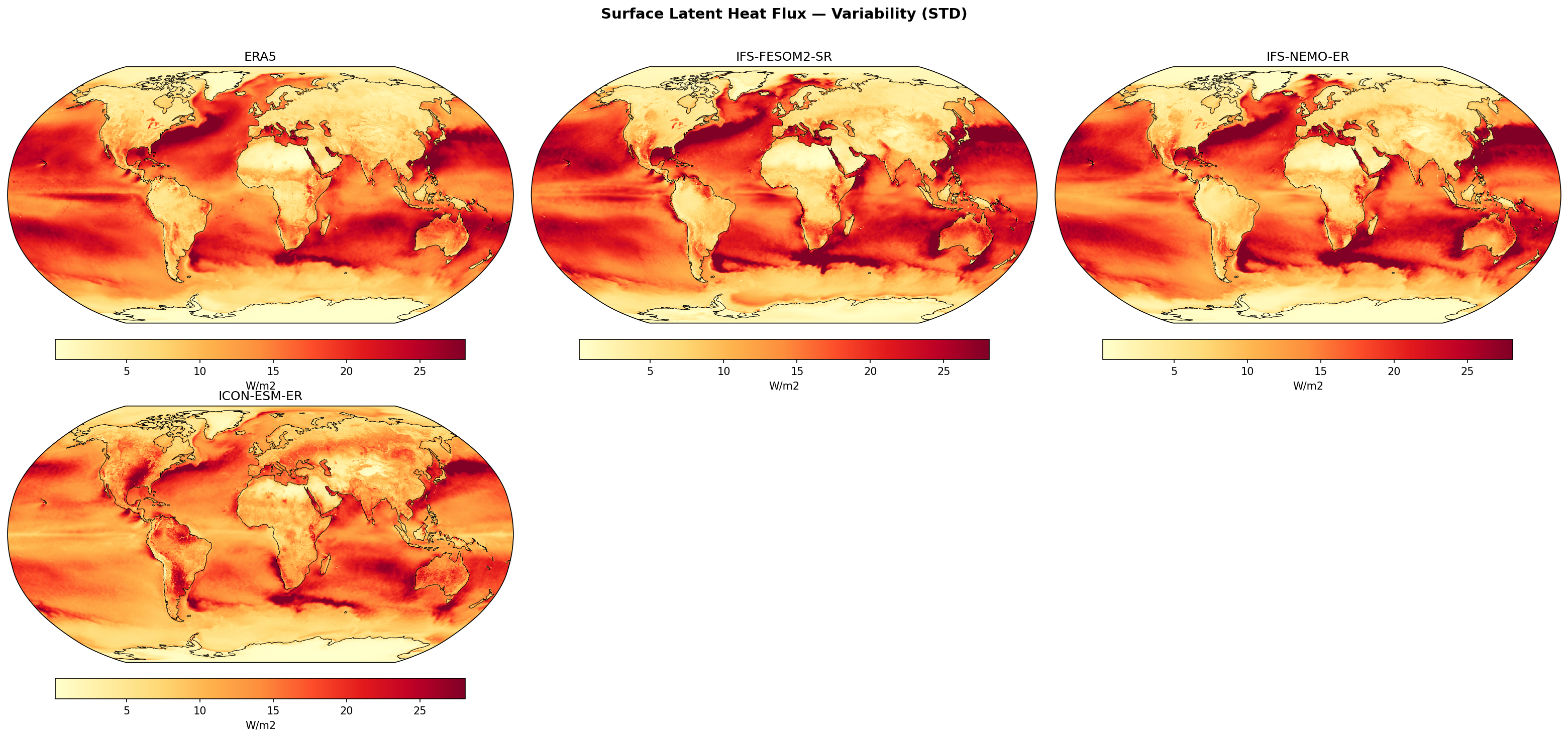
Surface Latent Heat Flux — Variability (STD)
| Variables | hfls |
|---|---|
| Models | IFS-FESOM2-SR, IFS-NEMO-ER, ICON-ESM-ER |
| Reference Dataset | ERA5 |
| Units | W/m2 |
| Period | 1980–2014 |
| IFS-FESOM2-SR | Std Gmean: 14.69 · Diff Gmean: 0.80 · Rmse: 3.34 |
| IFS-NEMO-ER | Std Gmean: 14.02 · Diff Gmean: 0.12 · Rmse: 2.94 |
| ICON-ESM-ER | Std Gmean: 13.14 · Diff Gmean: -0.75 · Rmse: 5.09 |
Summary high
This diagnostic compares the temporal variability (standard deviation) of surface latent heat flux in three high-resolution coupled models against ERA5 reanalysis. While all models capture the primary variability hotspots associated with Western Boundary Currents and tropical convection, the IFS-NEMO-ER model shows the closest statistical and spatial agreement with observations.
Key Findings
- IFS-NEMO-ER demonstrates the best performance with the lowest RMSE (2.94 W/m²) and a minimal global mean bias (+0.12 W/m²), closely replicating the intensity of variability in the Gulf Stream and Kuroshio extensions.
- IFS-FESOM2-SR tends to slightly overestimate variability globally (bias +0.80 W/m²), with visibly higher intensity in the Southern Ocean and tropical Pacific compared to ERA5.
- ICON-ESM-ER consistently underestimates variability (bias -0.75 W/m²) and exhibits the highest RMSE (5.09 W/m²), with notable deficiencies in reproducing the magnitude of variability over tropical oceans and major land basins like the Amazon.
Spatial Patterns
Dominant variability maxima (>25 W/m²) are located over Western Boundary Currents (Gulf Stream, Kuroshio, Agulhas), driven by strong air-sea temperature contrasts and storm activity, and over tropical warm pools (Indo-Pacific). Continental variability is highest over tropical rainforests (Amazon, Congo). Low variability (<5 W/m²) characterizes high-latitude ice regions and eastern subtropical upwelling zones.
Model Agreement
The two IFS-based models show strong structural agreement with ERA5, though IFS-FESOM2-SR is slightly more energetic. ICON-ESM-ER diverges more significantly, showing weaker variability contrasts, particularly over land (e.g., noticeably lower variability over South America) and in the Indian Ocean.
Physical Interpretation
Latent heat flux variability is primarily driven by fluctuations in wind speed and near-surface specific humidity gradients. The high-resolution ocean components (~10 km) in these models allow for the resolution of sharp SST fronts in Western Boundary Currents, which act as anchors for high flux variability during synoptic events. The reduced variability in ICON-ESM-ER may suggest damped surface exchange processes or weaker SST variability compared to the IFS configurations.
Caveats
- ERA5 reanalysis is used as the ground truth but relies on bulk aerodynamic formulas and model physics itself.
- The analysis does not distinguish between timescales (e.g., synoptic vs. interannual ENSO variability) within the 'deseasonalised' signal.
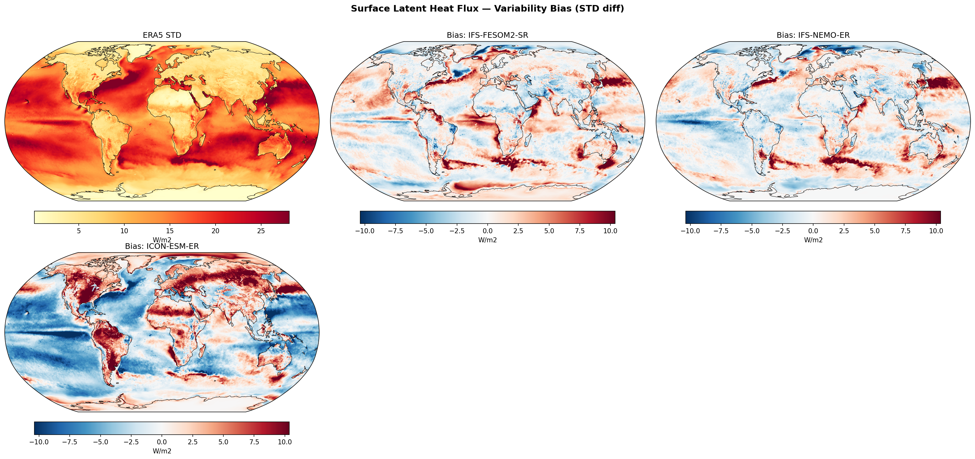
Surface Latent Heat Flux — Variability Bias (STD diff)
| Variables | hfls |
|---|---|
| Models | IFS-FESOM2-SR, IFS-NEMO-ER, ICON-ESM-ER |
| Reference Dataset | ERA5 |
| Units | W/m2 |
| Period | 1980–2014 |
| IFS-FESOM2-SR | Std Gmean: 14.69 · Diff Gmean: 0.80 · Rmse: 3.34 |
| IFS-NEMO-ER | Std Gmean: 14.02 · Diff Gmean: 0.12 · Rmse: 2.94 |
| ICON-ESM-ER | Std Gmean: 13.14 · Diff Gmean: -0.75 · Rmse: 5.09 |
Summary high
This diagnostic evaluates the variability (standard deviation) of Surface Latent Heat Flux in three high-resolution coupled models compared to ERA5 reanalysis. The IFS-based models exhibit enhanced variability in western boundary currents, whereas ICON-ESM-ER shows widespread underestimation of oceanic variability contrasted with excessive variability over tropical land.
Key Findings
- IFS-FESOM2-SR and IFS-NEMO-ER show strong positive variability biases (>5-10 W/m²) in Western Boundary Currents (Gulf Stream, Kuroshio) and the Agulhas Return Current, suggesting highly energetic ocean-atmosphere coupling in eddy-rich regions.
- ICON-ESM-ER systematically underestimates latent heat flux variability over most global oceans (global mean bias -0.75 W/m²), particularly in the Southern Ocean and subtropics.
- Conversely, ICON-ESM-ER exhibits strong positive variability biases over tropical land masses (Amazon, Congo Basin, Maritime Continent), indicating excessive volatility in terrestrial evapotranspiration or convective precipitation cycles.
- IFS-NEMO-ER has the lowest global RMSE (2.94 W/m²) and the smallest mean bias, showing the closest aggregate agreement with ERA5 variability patterns.
Spatial Patterns
ERA5 shows peak variability in WBCs and tropical oceans. The IFS models amplify this pattern in the WBCs but underestimate variability in eastern boundary upwelling zones (e.g., off Peru/Chile, California). ICON-ESM-ER displays a distinct land-sea contrast: widespread 'blue' (negative bias) over oceans and 'red' (positive bias) over tropical rainforests. Both IFS models show patches of positive bias in the Southern Ocean, whereas ICON shows strong negative bias there.
Model Agreement
The two IFS models (FESOM and NEMO) show high structural agreement, sharing similar bias patterns in WBCs and upwelling zones, likely driven by their common atmospheric component and similar ocean resolution. ICON-ESM-ER diverges significantly, being the outlier with opposite signs of bias over large oceanic regions and unique land biases.
Physical Interpretation
The positive bias in WBCs for IFS models likely reflects resolving mesoscale ocean eddies (~10 km resolution) which drive strong, transient air-sea flux anomalies that may exceed those in the ~31 km ERA5 reanalysis. The negative bias in eastern boundaries in IFS models suggests issues capturing the variability of coastal upwelling systems or overlying cloud decks. ICON's reduced oceanic variability suggests stronger damping of surface fluxes or insufficient wind-driven variability, while its land bias points to issues in the land-surface model (JSBACH) or coupling with convection (precip-evaporation feedback).
Caveats
- ERA5 is a reanalysis model itself; 'biases' in high-resolution models might partly reflect valid small-scale variability unresolved by ERA5.
- Differences in effective resolution between the models (particularly ocean grids) and the ERA5 grid may influence the amplitude of variability in sharp frontal regions.
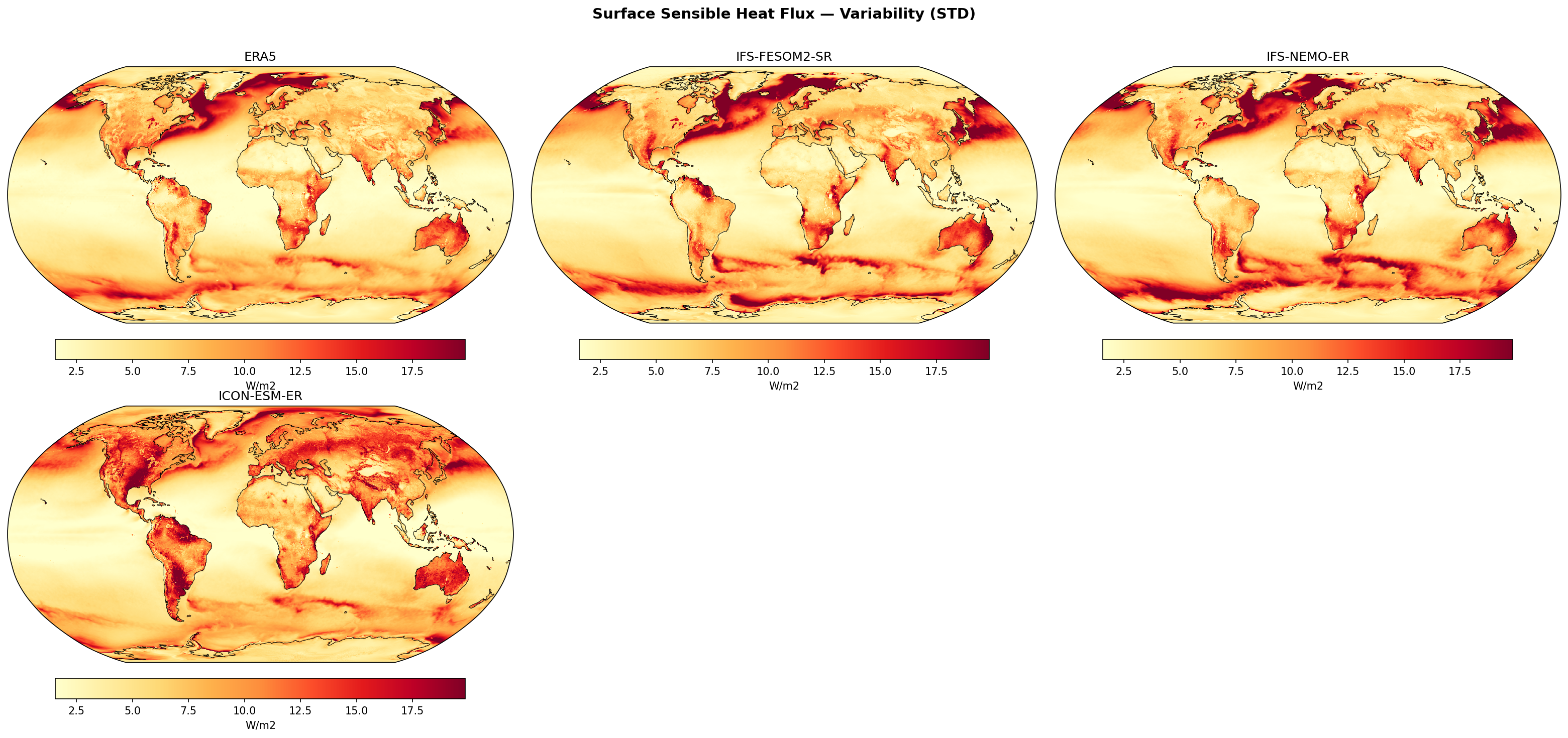
Surface Sensible Heat Flux — Variability (STD)
| Variables | hfss |
|---|---|
| Models | IFS-FESOM2-SR, IFS-NEMO-ER, ICON-ESM-ER |
| Reference Dataset | ERA5 |
| Units | W/m2 |
| Period | 1980–2014 |
| IFS-FESOM2-SR | Std Gmean: 6.45 · Diff Gmean: 0.49 · Rmse: 2.48 |
| IFS-NEMO-ER | Std Gmean: 6.57 · Diff Gmean: 0.61 · Rmse: 2.50 |
| ICON-ESM-ER | Std Gmean: 6.74 · Diff Gmean: 0.79 · Rmse: 3.43 |
Summary high
This diagnostic shows the standard deviation of deseasonalised, detrended monthly Surface Sensible Heat Flux (SSHF), highlighting regions of strong air-sea interaction and land-atmosphere coupling variability.
Key Findings
- High SSHF variability is concentrated in Western Boundary Currents (Gulf Stream, Kuroshio), marginal sea ice zones, and major continental landmasses.
- IFS-FESOM2-SR and IFS-NEMO-ER show excellent agreement with ERA5, with spatial patterns and global mean variability closely matching observations (RMSE ~2.5 W/m²).
- ICON-ESM-ER systematically overestimates SSHF variability over continental regions, particularly the Amazon, Central Africa, and Boreal forests, leading to the highest global RMSE (3.43 W/m²).
Spatial Patterns
Dominant variability features include the Gulf Stream and Kuroshio extensions (>15 W/m²), driven by sporadic cold air outbreaks over warm waters. The Marginal Ice Zones (e.g., Labrador Sea, Greenland Sea, Southern Ocean) also exhibit high variability due to fluctuations in sea ice extent exposing open water. Over land, variability is higher than over subtropical oceans, with notable hotspots in arid and semi-arid regions (Australia, Sahara) and the Amazon.
Model Agreement
The two IFS-based models (FESOM2 and NEMO) are visually very similar to each other and to ERA5, capturing both the magnitude and spatial distribution of variability accurately. ICON-ESM-ER captures the oceanic patterns relatively well (though slightly more diffuse in the North Atlantic) but diverges significantly over land, displaying excessive variability across South America, Africa, and Eurasia.
Physical Interpretation
Oceanic variability maxima coincide with regions of intense air-sea heat exchange: Western Boundary Currents where warm water meets cold continental air, and sea ice margins where surface properties switch between insulating ice and open water. The land bias in ICON-ESM-ER suggests overly sensitive land-atmosphere coupling or issues in the land surface scheme (JSBACH) parameterizations for soil moisture or surface roughness, leading to exaggerated fluctuations in surface fluxes.
Caveats
- Analysis uses monthly mean data, which filters out high-frequency synoptic variability (daily timescales) relevant for sensible heat extremes.
- Reference data is ERA5, which is a reanalysis product and relies on its own model physics for surface fluxes, though constrained by observations.
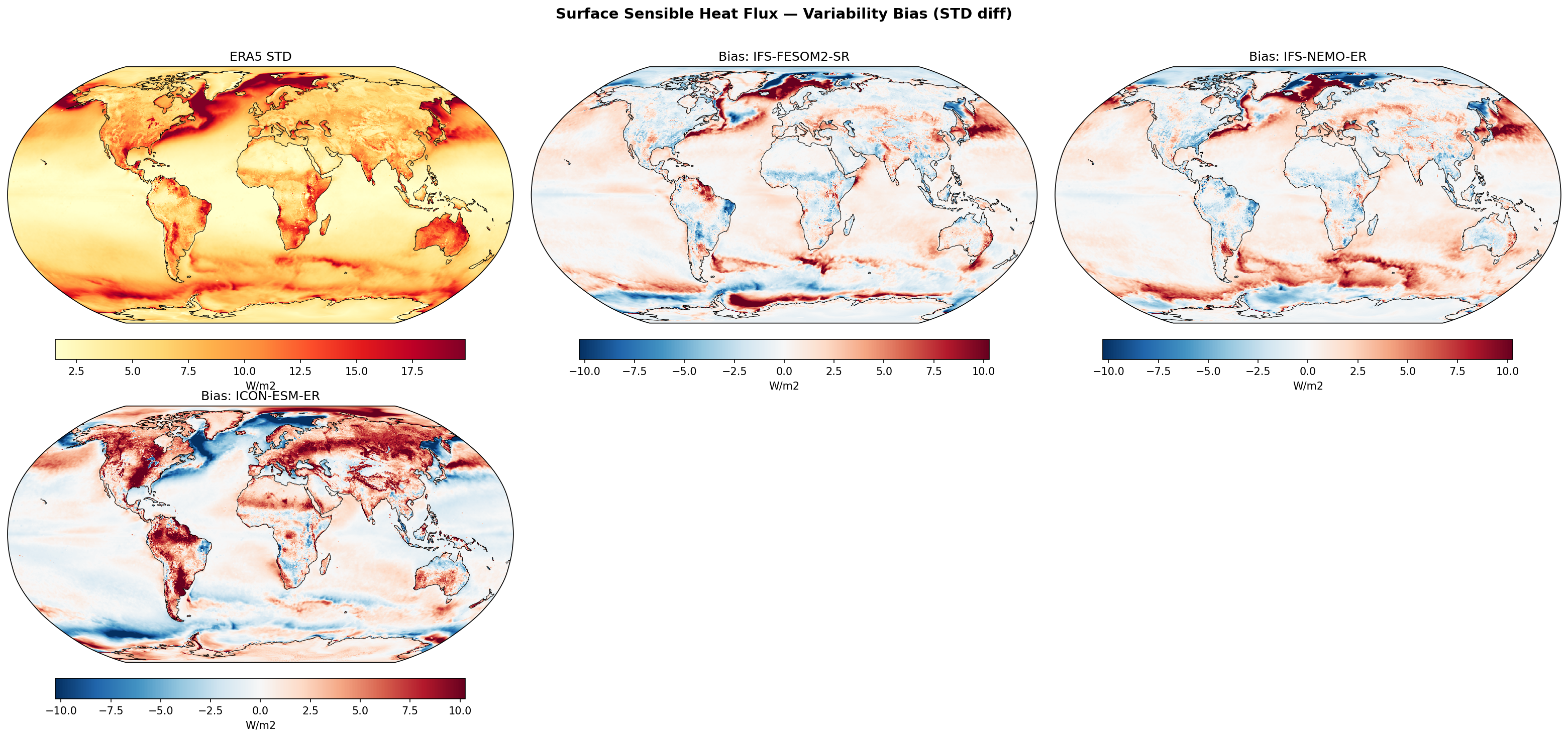
Surface Sensible Heat Flux — Variability Bias (STD diff)
| Variables | hfss |
|---|---|
| Models | IFS-FESOM2-SR, IFS-NEMO-ER, ICON-ESM-ER |
| Reference Dataset | ERA5 |
| Units | W/m2 |
| Period | 1980–2014 |
| IFS-FESOM2-SR | Std Gmean: 6.45 · Diff Gmean: 0.49 · Rmse: 2.48 |
| IFS-NEMO-ER | Std Gmean: 6.57 · Diff Gmean: 0.61 · Rmse: 2.50 |
| ICON-ESM-ER | Std Gmean: 6.74 · Diff Gmean: 0.79 · Rmse: 3.43 |
Summary high
This diagnostic evaluates the variability (standard deviation) of Surface Sensible Heat Flux (SSHF) in three high-resolution coupled models compared to ERA5 reanalysis. The IFS-based models exhibit similar oceanic biases, particularly in western boundary currents, while ICON-ESM-ER is an outlier with excessive variability over land.
Key Findings
- IFS-FESOM2-SR and IFS-NEMO-ER show strong positive variability biases (>5 W/m²) in the Gulf Stream and Kuroshio extensions, suggesting more energetic air-sea interaction in these eddy-rich regions than ERA5.
- ICON-ESM-ER exhibits widespread, high-magnitude positive variability biases over global landmasses (North America, Eurasia, Amazon), leading to a significantly higher global RMSE (3.43 W/m²) compared to the IFS models (~2.5 W/m²).
- All models display distinct dipole bias patterns in the Southern Ocean and high-latitude North Atlantic, indicative of mismatches in sea ice edge location and variability.
- IFS-NEMO-ER and IFS-FESOM2-SR show remarkable similarity, implying that the atmospheric component (IFS) dominates the sensible heat flux characteristics rather than the specific ocean discretization.
Spatial Patterns
ERA5 shows peak SSHF variability in Western Boundary Currents and marginal ice zones. The IFS models replicate this but with higher magnitude in the boundary currents. In the Southern Ocean, models show concentric bands of positive and negative bias, reflecting errors in the meridional oscillation of the sea ice edge. ICON is distinct for its continental red bias (excess variability) and blue bias (reduced variability) in the North Atlantic subpolar gyre and Weddell Sea.
Model Agreement
High agreement between the two IFS variants (FESOM vs NEMO) suggests robust behavior of the IFS atmospheric physics. ICON diverges significantly, particularly over land and in the North Atlantic, showing lower agreement with observations in these domains.
Physical Interpretation
The positive bias in Western Boundary Currents for IFS models likely stems from resolved mesoscale ocean eddies and sharp SST fronts driving intense turbulent flux variability, which may be smoothed in the ERA5 reanalysis. ICON's excessive land variability points to potential issues in the land surface model (JSBACH) or land-atmosphere coupling, possibly related to surface skin temperature or soil moisture volatility. The sea ice zone biases arise because the phase change between insulating ice and open water creates massive heat flux differences; slight spatial offsets in the ice edge climatology or variance result in large local flux errors.
Caveats
- ERA5 is a reanalysis model and may lack the effective resolution to capture the peak variability of sharp SST fronts in Western Boundary Currents, meaning positive model bias here could partly represent added value.
- The strong land bias in ICON dominates the global statistics, potentially obscuring ocean performance in global metrics.
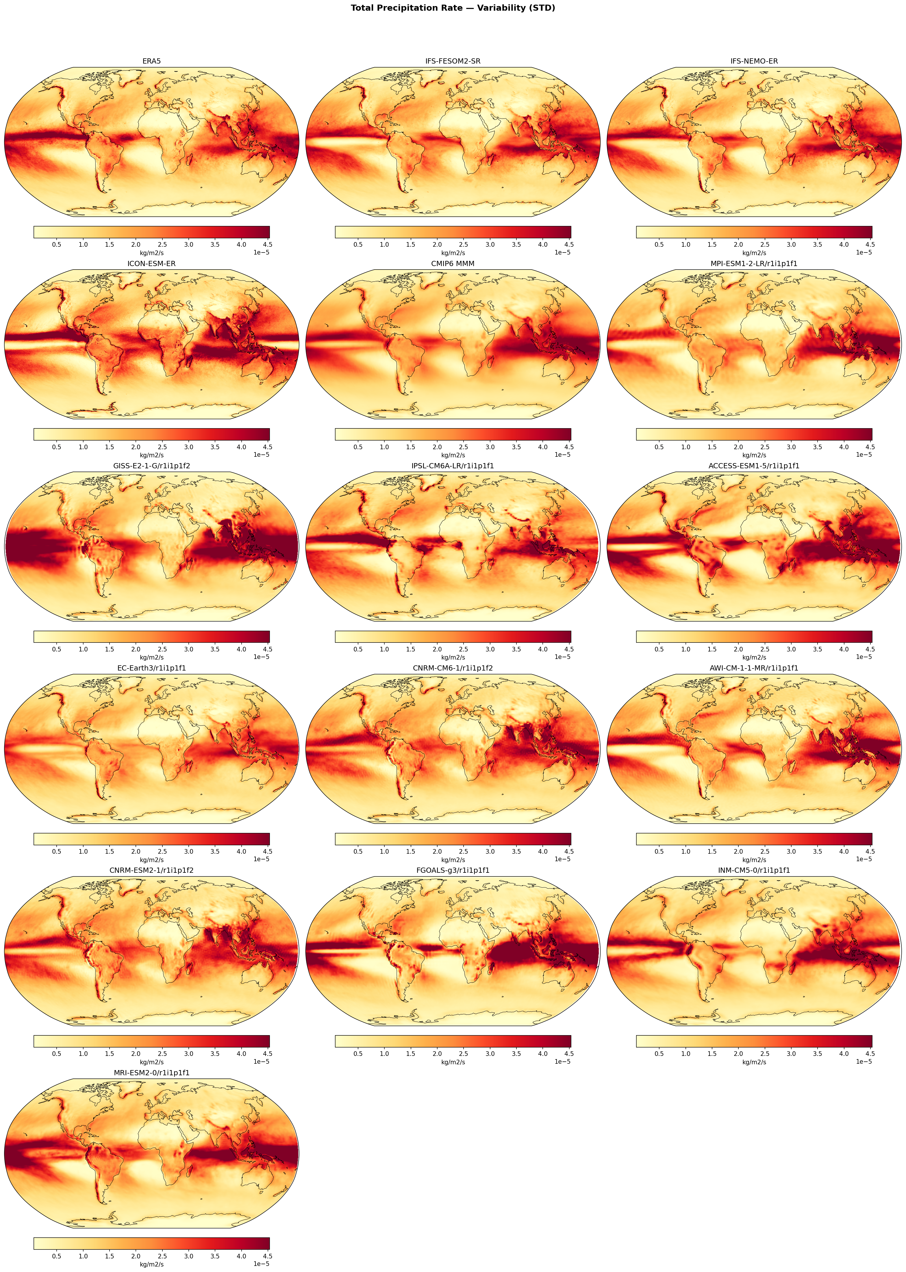
Total Precipitation Rate — Variability (STD)
| Variables | pr |
|---|---|
| Models | IFS-FESOM2-SR, IFS-NEMO-ER, ICON-ESM-ER, CMIP6 MMM, MPI-ESM1-2-LR/r1i1p1f1, GISS-E2-1-G/r1i1p1f2, IPSL-CM6A-LR/r1i1p1f1, ACCESS-ESM1-5/r1i1p1f1, EC-Earth3/r1i1p1f1, CNRM-CM6-1/r1i1p1f2, AWI-CM-1-1-MR/r1i1p1f1, CNRM-ESM2-1/r1i1p1f2, FGOALS-g3/r1i1p1f1, INM-CM5-0/r1i1p1f1, MRI-ESM2-0/r1i1p1f1 |
| Reference Dataset | ERA5 |
| Units | kg/m2/s |
| Period | 1980–2014 |
| IFS-FESOM2-SR | Std Gmean: 0.00 · Diff Gmean: 0.00 · Rmse: 0.00 |
| IFS-NEMO-ER | Std Gmean: 0.00 · Diff Gmean: -0.00 · Rmse: 0.00 |
| ICON-ESM-ER | Std Gmean: 0.00 · Diff Gmean: 0.00 · Rmse: 0.00 |
| CMIP6 MMM | Std Gmean: 0.00 · Diff Gmean: 0.00 · Rmse: 0.00 |
Summary high
This diagnostic compares the standard deviation of deseasonalised, detrended monthly total precipitation rates across high-resolution EERIE models (IFS and ICON), the CMIP6 Multi-Model Mean (MMM), and individual CMIP6 models against ERA5 reanalysis (1980–2014). The maps highlight regions of high hydrological variability, primarily associated with the ITCZ, SPCZ, Asian Monsoon, and mid-latitude storm tracks.
Key Findings
- IFS-NEMO-ER demonstrates the best agreement with ERA5, achieving the lowest RMSE (4.41e-6 kg/m²/s) and faithfully reproducing the spatial structure of tropical and mid-latitude variability.
- ICON-ESM-ER significantly overestimates precipitation variability globally (std_gmean ~1.91e-5 vs ~1.52e-5 in IFS-NEMO), with excessive variance concentrated in the tropical Pacific and Indian Ocean.
- While many CMIP6 models (e.g., FGOALS-g3, GISS-E2-1-G) display distinct 'double ITCZ' biases in their variability patterns, the IFS-based EERIE models largely avoid this, maintaining a realistic separation between the ITCZ and SPCZ.
- IFS-FESOM2-SR captures spatial patterns well but has a slightly higher RMSE than the NEMO coupled version, showing somewhat higher variability in the tropical Pacific.
Spatial Patterns
Dominant variability is found in the tropical convection zones (ITCZ, SPCZ, Indo-Pacific Warm Pool) and the North Atlantic/Pacific storm tracks. The subtropics show characteristic low variability. ERA5 shows a sharp, narrow ITCZ band; ICON-ESM-ER broadens and intensifies this feature, while several CMIP6 models show a zonal band in the southern tropical Pacific indicative of a double ITCZ.
Model Agreement
The IFS variants (FESOM and NEMO) agree well with ERA5 in terms of pattern and magnitude. There is substantial divergence among CMIP6 models: GISS and ACCESS show extremely high variability, while INM-CM5-0 is notably dampened. ICON-ESM-ER is an outlier among the high-res models, showing excessive 'hotspots' of variability.
Physical Interpretation
High precipitation variability in the tropics is driven by deep convection dynamics, ENSO-related shifts, and monsoon systems. The excessive variability in ICON-ESM-ER suggests overly sensitive convective parameterizations or strong local coupling feedbacks that amplify hydro-meteorological fluctuations. The fidelity of the IFS models implies that their resolution and physics tuning effectively capture the statistics of synoptic and intraseasonal precipitation events without the exaggerated feedback seen in some CMIP6 members.
Caveats
- ERA5 precipitation is a model-derived forecast product within the reanalysis and has its own uncertainties, particularly over open oceans.
- The analysis is based on detrended data, so it reflects internal variability (interannual/decadal) rather than long-term climate change signals.
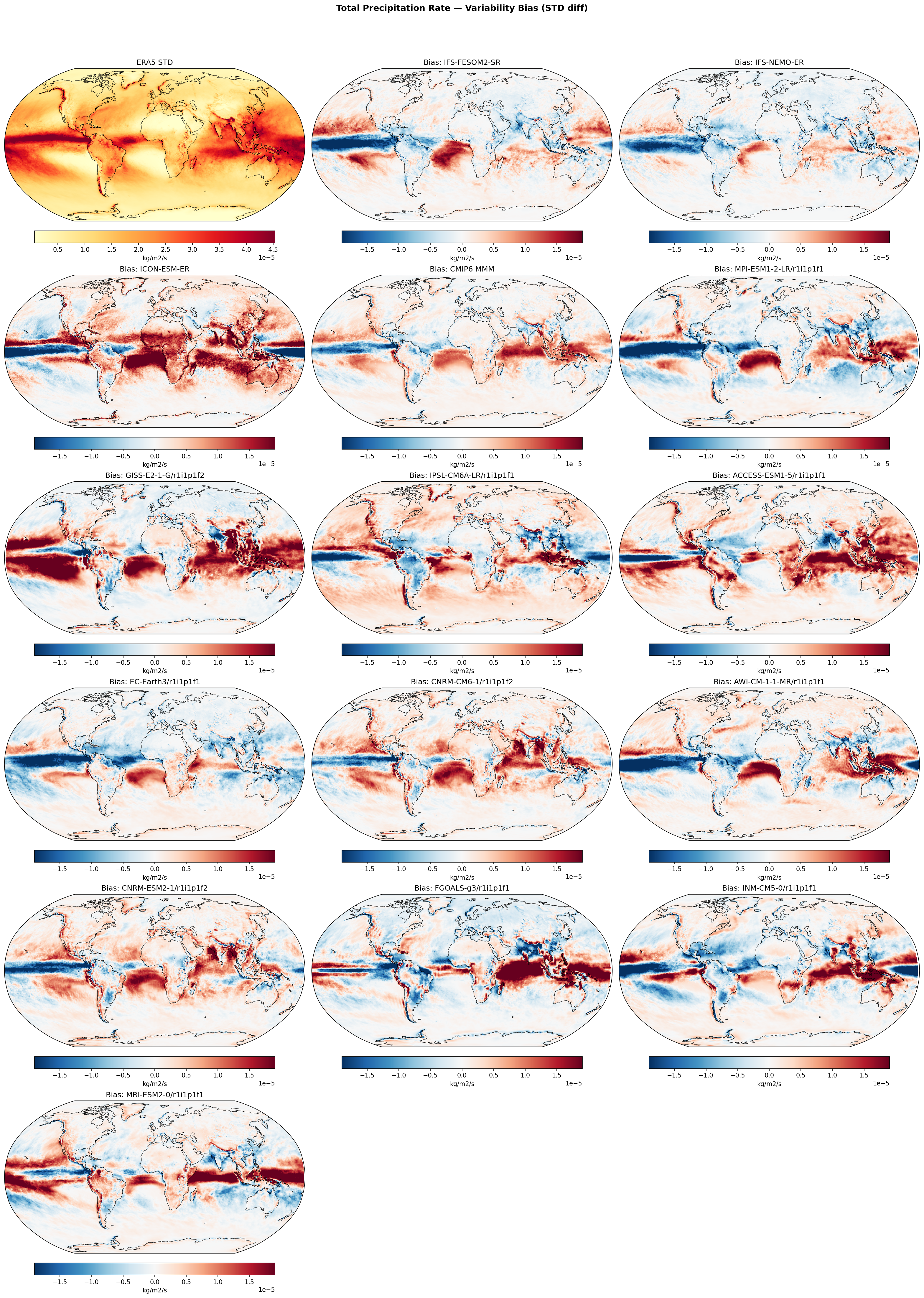
Total Precipitation Rate — Variability Bias (STD diff)
| Variables | pr |
|---|---|
| Models | IFS-FESOM2-SR, IFS-NEMO-ER, ICON-ESM-ER, CMIP6 MMM, MPI-ESM1-2-LR/r1i1p1f1, GISS-E2-1-G/r1i1p1f2, IPSL-CM6A-LR/r1i1p1f1, ACCESS-ESM1-5/r1i1p1f1, EC-Earth3/r1i1p1f1, CNRM-CM6-1/r1i1p1f2, AWI-CM-1-1-MR/r1i1p1f1, CNRM-ESM2-1/r1i1p1f2, FGOALS-g3/r1i1p1f1, INM-CM5-0/r1i1p1f1, MRI-ESM2-0/r1i1p1f1 |
| Reference Dataset | ERA5 |
| Units | kg/m2/s |
| Period | 1980–2014 |
| IFS-FESOM2-SR | Std Gmean: 0.00 · Diff Gmean: 0.00 · Rmse: 0.00 |
| IFS-NEMO-ER | Std Gmean: 0.00 · Diff Gmean: -0.00 · Rmse: 0.00 |
| ICON-ESM-ER | Std Gmean: 0.00 · Diff Gmean: 0.00 · Rmse: 0.00 |
| CMIP6 MMM | Std Gmean: 0.00 · Diff Gmean: 0.00 · Rmse: 0.00 |
Summary high
This figure evaluates the variability (standard deviation of anomalies) of the Total Precipitation Rate across EERIE high-resolution models and CMIP6 compared to ERA5. The IFS models generally underestimate equatorial precipitation variability, whereas ICON-ESM-ER and many CMIP6 models strongly overestimate it.
Key Findings
- IFS-NEMO-ER and IFS-FESOM2-SR exhibit a distinct negative bias (blue bands) along the equatorial Pacific and Atlantic, indicating suppressed precipitation variability in the ITCZ core.
- ICON-ESM-ER shows a widespread positive bias (red) throughout the tropics, particularly in the ITCZ, SPCZ, and Indian Ocean, suggesting an overly active hydrological cycle or sensitive convection scheme.
- The CMIP6 Multi-Model Mean (MMM) and several individual models display a characteristic 'double ITCZ' bias pattern: negative variability bias on the equator flanked by positive biases, indicating displaced storm tracks.
- IFS-NEMO-ER achieves the lowest global RMSE (4.41e-6 kg/m²/s) among the featured models, slightly outperforming the CMIP6 MMM (4.90e-6 kg/m²/s).
Spatial Patterns
ERA5 shows peak precipitation variability in the Western Pacific Warm Pool, ITCZ, and SPCZ. The models struggle primarily in the tropics: IFS variants show a zonal band of underestimation along the equator (0°N). In contrast, ICON and models like GISS-E2-1-G show broad regions of overestimation in the tropical Pacific and Indian Ocean. Extratropical storm track variability is generally better captured, with smaller amplitude biases.
Model Agreement
There is significant divergence between the high-resolution models. The two IFS-based models (NEMO and FESOM) agree on the sign of the bias (negative/underestimation in the deep tropics), while ICON-ESM-ER stands apart with a strong positive bias. The IFS models align better with the low-variability tendency seen in ERA5 compared to the high-variability outliers in the CMIP6 ensemble (e.g., ACCESS, GISS).
Physical Interpretation
Precipitation variability biases are closely linked to mean-state errors and ENSO dynamics. The negative bias along the equator in IFS models likely reflects a 'cold tongue' bias or suppressed deep convection preventing realistic ENSO-driven rainfall variability. The 'off-equator positive / on-equator negative' pattern in CMIP6 MMM confirms that displaced mean precipitation bands (Double ITCZ) also displace the associated variability. ICON's widespread high variability suggests a convection parameterization that triggers too frequently or strongly.
Caveats
- ERA5 precipitation is a reanalysis product (model-derived) and not direct observation, though it assimilates vast amounts of data.
- The analysis does not distinguish between timescales (e.g., intra-seasonal vs. inter-annual), so it bundles MJO and ENSO variability together.
Mean Sea Level Pressure — Variability (STD)
| Variables | psl |
|---|---|
| Models | IFS-FESOM2-SR, IFS-NEMO-ER, ICON-ESM-ER, CMIP6 MMM, MPI-ESM1-2-LR/r1i1p1f1, GISS-E2-1-G/r1i1p1f2, IPSL-CM6A-LR/r1i1p1f1, ACCESS-ESM1-5/r1i1p1f1, EC-Earth3/r1i1p1f1, CNRM-CM6-1/r1i1p1f2, AWI-CM-1-1-MR/r1i1p1f1, CNRM-ESM2-1/r1i1p1f2, FGOALS-g3/r1i1p1f1, INM-CM5-0/r1i1p1f1, MRI-ESM2-0/r1i1p1f1 |
| Reference Dataset | ERA5 |
| Units | Pa |
| Period | 1980–2014 |
| IFS-FESOM2-SR | Std Gmean: 239.35 · Diff Gmean: 3.56 · Rmse: 24.18 |
| IFS-NEMO-ER | Std Gmean: 239.05 · Diff Gmean: 3.26 · Rmse: 19.96 |
| ICON-ESM-ER | Std Gmean: 228.37 · Diff Gmean: -7.41 · Rmse: 32.64 |
| CMIP6 MMM | Std Gmean: 249.90 · Diff Gmean: 14.19 · Rmse: 26.38 |
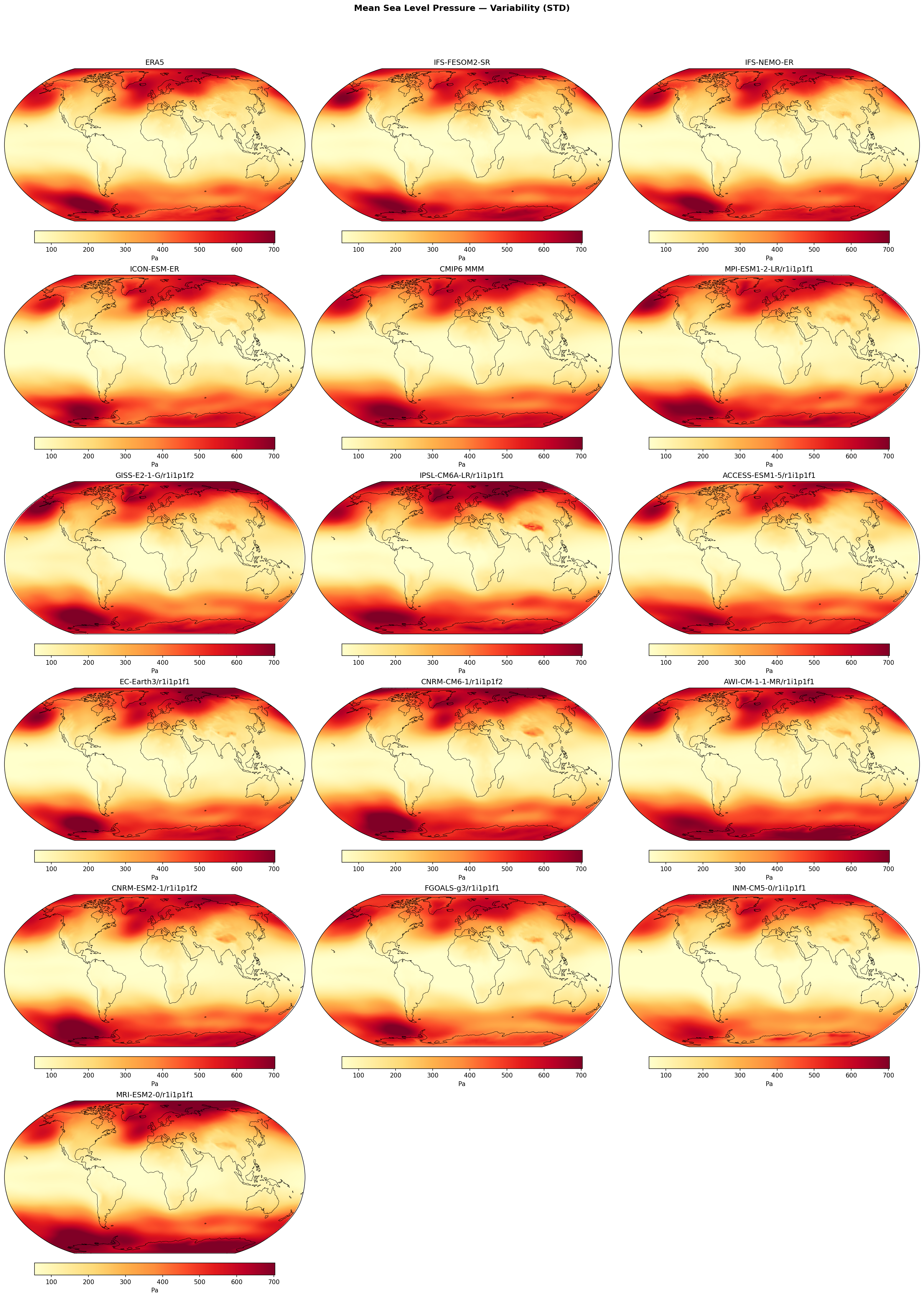
Summary high
This figure displays the standard deviation of deseasonalised, detrended monthly Mean Sea Level Pressure (MSLP), acting as a proxy for low-frequency atmospheric variability and storm track activity. The high-resolution IFS models show excellent agreement with ERA5, while ICON-ESM-ER slightly underestimates variability and the CMIP6 ensemble exhibits large inter-model spread.
Key Findings
- IFS-NEMO-ER and IFS-FESOM2-SR capture the spatial patterns and magnitude of MSLP variability with high fidelity, showing the lowest RMSE values (19.96 Pa and 24.18 Pa, respectively).
- ICON-ESM-ER systematically underestimates global MSLP variability (bias of -7.4 Pa), visible as weaker intensities in the major storm tracks compared to ERA5.
- The CMIP6 Multi-Model Mean (MMM) overestimates global variability (bias +14.2 Pa), driven by individual models like ACCESS-ESM1-5 and CNRM-CM6-1 which show much higher variability intensities than observations.
- Individual CMIP6 models show significant diversity, ranging from the low-variability INM-CM5-0 to the high-variability EC-Earth3 and CNRM models, contrasting with the tighter consistency of the high-resolution EERIE models.
Spatial Patterns
Dominant variability maxima (>600 Pa) are located in the Southern Ocean circumpolar trough and the Northern Hemisphere storm tracks (North Atlantic and North Pacific). The North Atlantic track exhibits a characteristic northeastward tilt towards Scandinavia. Tropical regions show minimal variability (<200 Pa).
Model Agreement
IFS-NEMO-ER shows the best agreement with ERA5, followed closely by IFS-FESOM2-SR. ICON-ESM-ER reproduces the spatial structure well but lacks amplitude. CMIP6 models vary widely, with the MMM suggesting a general overestimation of extratropical variability compared to the high-resolution simulations and ERA5.
Physical Interpretation
The patterns reflect the regions of highest synoptic eddy activity and low-frequency variability modes (e.g., NAO, PNA, SAM). The variability in monthly means captures the aggregate effect of storm systems and blocking events. The superior performance of IFS models suggests that their resolution and tuning successfully capture the energetics of these mid-latitude systems, whereas the spread in CMIP6 indicates varying degrees of storm track dampening or hyperactivity.
Caveats
- Analysis is based on monthly means, which smooths out high-frequency synoptic variability (daily timescales).
- Units are in Pascals (Pa); 500 Pa corresponds to 5 hPa.
Mean Sea Level Pressure — Variability Bias (STD diff)
| Variables | psl |
|---|---|
| Models | IFS-FESOM2-SR, IFS-NEMO-ER, ICON-ESM-ER, CMIP6 MMM, MPI-ESM1-2-LR/r1i1p1f1, GISS-E2-1-G/r1i1p1f2, IPSL-CM6A-LR/r1i1p1f1, ACCESS-ESM1-5/r1i1p1f1, EC-Earth3/r1i1p1f1, CNRM-CM6-1/r1i1p1f2, AWI-CM-1-1-MR/r1i1p1f1, CNRM-ESM2-1/r1i1p1f2, FGOALS-g3/r1i1p1f1, INM-CM5-0/r1i1p1f1, MRI-ESM2-0/r1i1p1f1 |
| Reference Dataset | ERA5 |
| Units | Pa |
| Period | 1980–2014 |
| IFS-FESOM2-SR | Std Gmean: 239.35 · Diff Gmean: 3.56 · Rmse: 24.18 |
| IFS-NEMO-ER | Std Gmean: 239.05 · Diff Gmean: 3.26 · Rmse: 19.96 |
| ICON-ESM-ER | Std Gmean: 228.37 · Diff Gmean: -7.41 · Rmse: 32.64 |
| CMIP6 MMM | Std Gmean: 249.90 · Diff Gmean: 14.19 · Rmse: 26.38 |
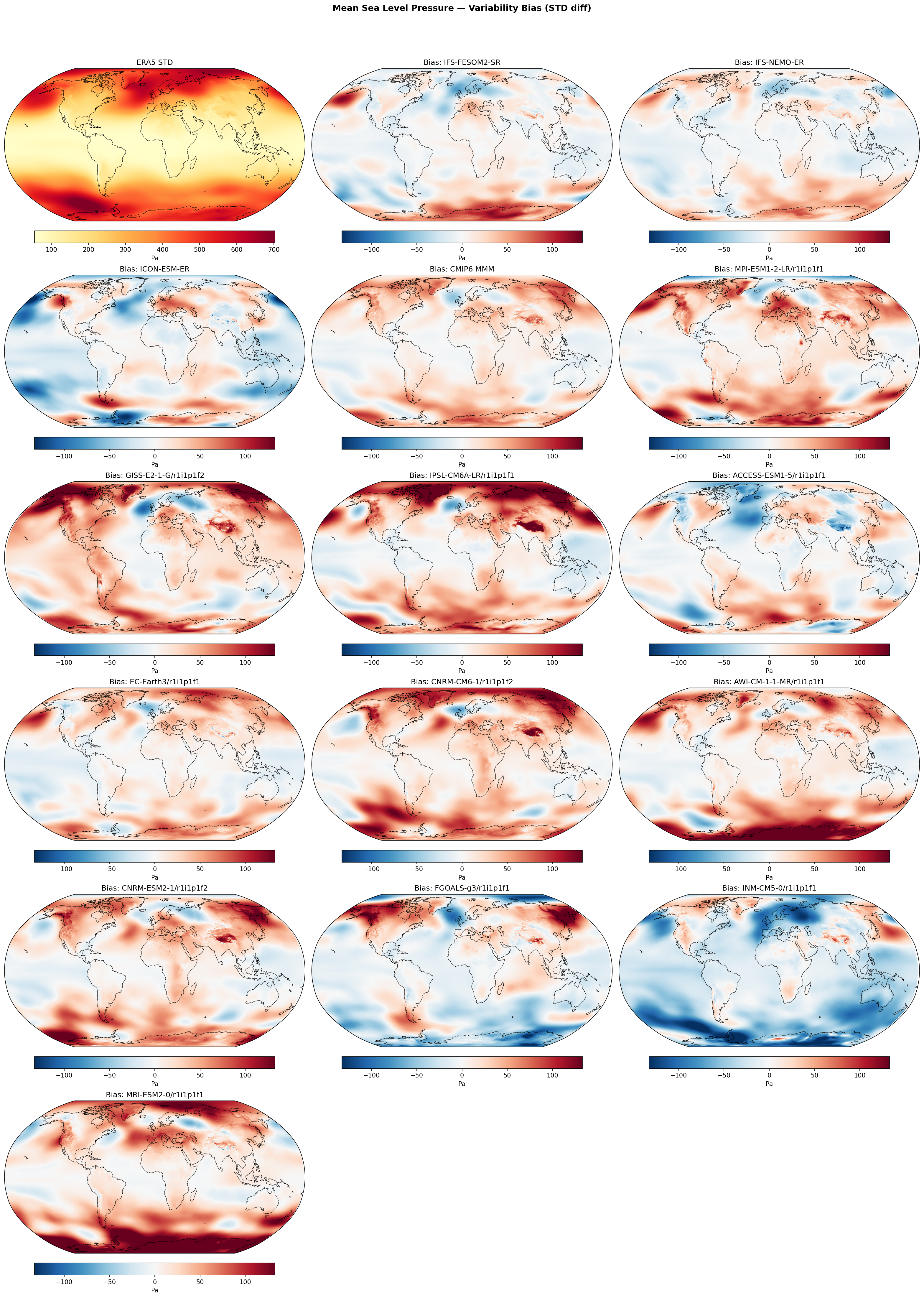
Summary high
This diagnostic evaluates the variability of Mean Sea Level Pressure (MSLP), a proxy for storm track activity, by comparing the standard deviation (STD) of deseasonalised anomalies in models versus ERA5.
Key Findings
- IFS-NEMO-ER performs best among the displayed models, with the lowest global RMSE (19.96 Pa) and very weak bias patterns, closely matching ERA5 variability.
- ICON-ESM-ER systematically underestimates MSLP variability (negative bias) in the major oceanic storm tracks (North Pacific and Southern Ocean), contrasting with the IFS models.
- The CMIP6 Multi-Model Mean and many individual CMIP6 models (e.g., CNRM, IPSL, GISS) tend to overestimate variability in high latitudes (Arctic and Southern Ocean), whereas INM-CM5-0 stands out with a strong global underestimation.
- IFS-FESOM2-SR shows slightly higher variability than IFS-NEMO-ER in the Southern Ocean but remains much closer to observations than the CMIP6 ensemble.
Spatial Patterns
ERA5 shows peak variability (>600 Pa) in the Aleutian Low, Icelandic Low, and the Southern Ocean circumpolar trough. The CMIP6 ensemble generally exhibits positive biases (red) in these regions and the Arctic, indicating excessive synoptic variance. ICON-ESM-ER displays zonal bands of negative bias (blue) in the Southern Hemisphere (40°S-60°S) and North Pacific. The IFS models show patchy, low-magnitude biases, with some localized positive bias in the Amundsen/Ross Sea sector.
Model Agreement
There is a distinct divergence between the high-resolution EERIE models: IFS variants agree well with observations, while ICON underestimates variability. The CMIP6 ensemble shows large inter-model spread, ranging from severe underestimation (INM-CM5-0) to widespread overestimation (CNRM-CM6-1, GISS-E2-1-G), with the ensemble mean leaning towards overestimation.
Physical Interpretation
MSLP standard deviation primarily captures the intensity and frequency of synoptic-scale cyclones (storm tracks). The positive biases in many CMIP6 models suggest storm tracks that are either too active, too deep, or meridionally displaced. The underestimation in ICON-ESM-ER suggests dampened synoptic activity or weaker cyclones in the storm tracks. The high fidelity of the IFS models implies that their resolution and physics parametrizations successfully capture the energy of atmospheric disturbances without the excessive noise seen in lower-resolution counterparts.
Caveats
- Standard deviation metrics do not distinguish between frequency and intensity of events, only total variance.
- Biases in the Arctic (CMIP6) may also relate to surface coupling over sea ice.
Surface Downwelling Longwave — Variability (STD)
| Variables | rlds |
|---|---|
| Models | IFS-FESOM2-SR, IFS-NEMO-ER, ICON-ESM-ER, CMIP6 MMM, MPI-ESM1-2-LR/r1i1p1f1, GISS-E2-1-G/r1i1p1f2, IPSL-CM6A-LR/r1i1p1f1, ACCESS-ESM1-5/r1i1p1f1, EC-Earth3/r1i1p1f1, CNRM-CM6-1/r1i1p1f2, AWI-CM-1-1-MR/r1i1p1f1, CNRM-ESM2-1/r1i1p1f2, FGOALS-g3/r1i1p1f1, INM-CM5-0/r1i1p1f1, MRI-ESM2-0/r1i1p1f1 |
| Reference Dataset | ERA5 |
| Units | W/m2 |
| Period | 1980–2014 |
| IFS-FESOM2-SR | Std Gmean: 7.48 · Diff Gmean: 0.31 · Rmse: 1.11 |
| IFS-NEMO-ER | Std Gmean: 7.31 · Diff Gmean: 0.14 · Rmse: 0.99 |
| ICON-ESM-ER | Std Gmean: 6.72 · Diff Gmean: -0.45 · Rmse: 1.74 |
| CMIP6 MMM | Std Gmean: 8.11 · Diff Gmean: 0.94 · Rmse: 1.34 |
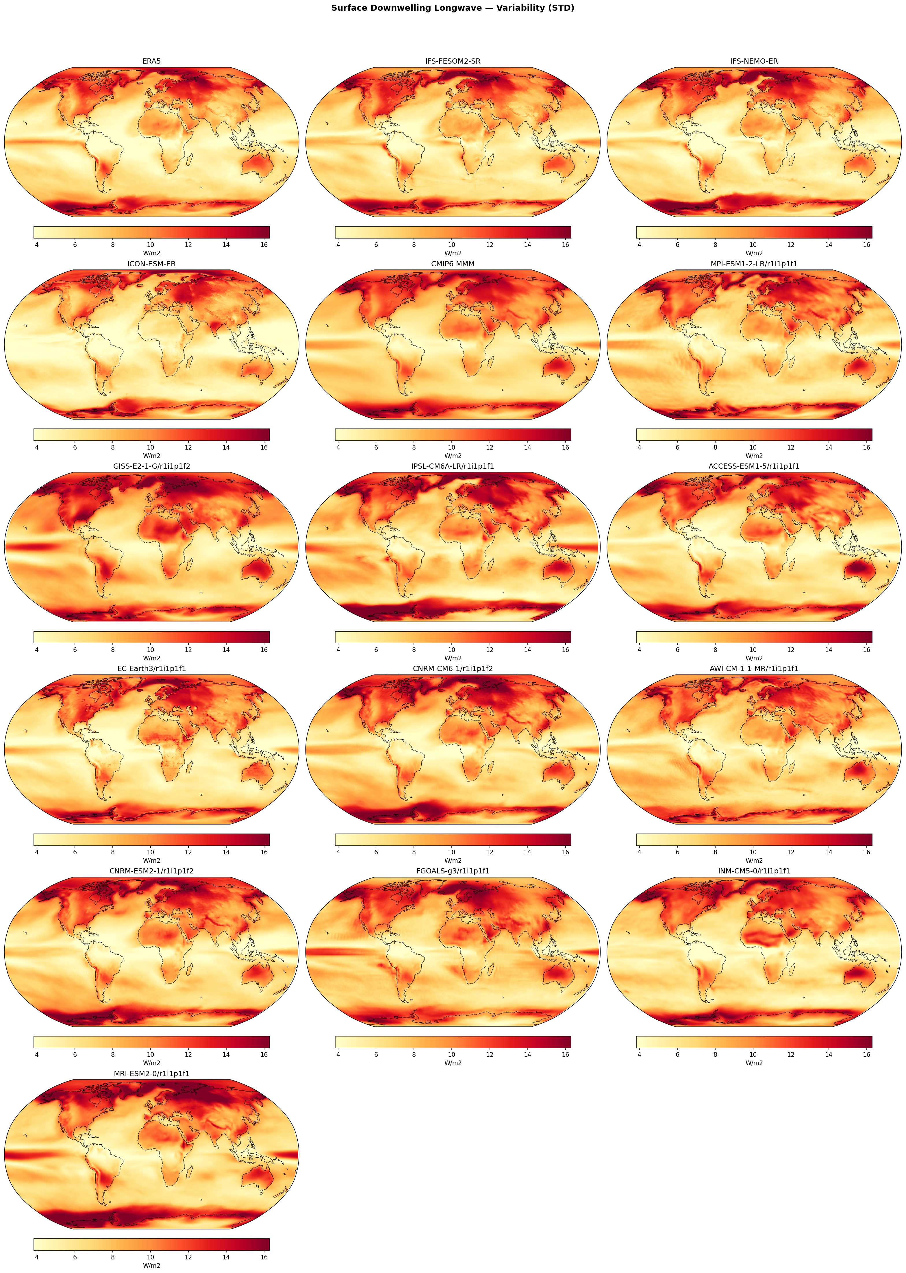
Summary high
This figure displays the standard deviation of deseasonalised, detrended monthly surface downwelling longwave radiation (rlds), illustrating the magnitude of internal climate variability across models compared to ERA5.
Key Findings
- IFS-NEMO-ER and IFS-FESOM2-SR show excellent agreement with ERA5, capturing both the spatial patterns and magnitude of variability (RMSE ~1.0-1.1 W/m²).
- ICON-ESM-ER systematically underestimates variability globally (negative bias of -0.45 W/m²), appearing noticeably paler than observations.
- The CMIP6 Multi-Model Mean (MMM) and several individual CMIP6 models (e.g., GISS-E2-1-G) tend to overestimate variability compared to ERA5 (MMM bias +0.94 W/m²).
Spatial Patterns
Variability is highest (>14 W/m²) over Northern Hemisphere continents (Siberia, North America) and the Southern Ocean, corresponding to regions of strong synoptic temperature variance and storm track activity. Variability is lowest (<6 W/m²) in the subtropical ocean gyres where subsidence creates stable atmospheric conditions.
Model Agreement
The high-resolution IFS models (NEMO and FESOM) outperform the ICON-ESM-ER and the CMIP6 MMM in reproducing the intensity of variability. IFS-NEMO-ER has the lowest RMSE (0.99 W/m²). Individual CMIP6 models show large dispersion, with GISS-E2-1-G showing excessive variability over oceans.
Physical Interpretation
Downwelling longwave variability is driven by fluctuations in near-surface air temperature and cloud cover (emissivity). High variability over land reflects the rapid thermal response of the land surface to synoptic weather systems (cold/warm fronts). The Southern Ocean band reflects storm track cloudiness variability. The underestimation in ICON suggests dampened synoptic activity or insufficient cloud variability.
Caveats
- GISS-E2-1-G appears to be an outlier with unrealistically high variability over global oceans.
- CMIP6 MMM smoothness usually dampens variability, but here the metric (mean of standard deviations) preserves the high variability bias of constituent models.
Surface Downwelling Longwave — Variability Bias (STD diff)
| Variables | rlds |
|---|---|
| Models | IFS-FESOM2-SR, IFS-NEMO-ER, ICON-ESM-ER, CMIP6 MMM, MPI-ESM1-2-LR/r1i1p1f1, GISS-E2-1-G/r1i1p1f2, IPSL-CM6A-LR/r1i1p1f1, ACCESS-ESM1-5/r1i1p1f1, EC-Earth3/r1i1p1f1, CNRM-CM6-1/r1i1p1f2, AWI-CM-1-1-MR/r1i1p1f1, CNRM-ESM2-1/r1i1p1f2, FGOALS-g3/r1i1p1f1, INM-CM5-0/r1i1p1f1, MRI-ESM2-0/r1i1p1f1 |
| Reference Dataset | ERA5 |
| Units | W/m2 |
| Period | 1980–2014 |
| IFS-FESOM2-SR | Std Gmean: 7.48 · Diff Gmean: 0.31 · Rmse: 1.11 |
| IFS-NEMO-ER | Std Gmean: 7.31 · Diff Gmean: 0.14 · Rmse: 0.99 |
| ICON-ESM-ER | Std Gmean: 6.72 · Diff Gmean: -0.45 · Rmse: 1.74 |
| CMIP6 MMM | Std Gmean: 8.11 · Diff Gmean: 0.94 · Rmse: 1.34 |
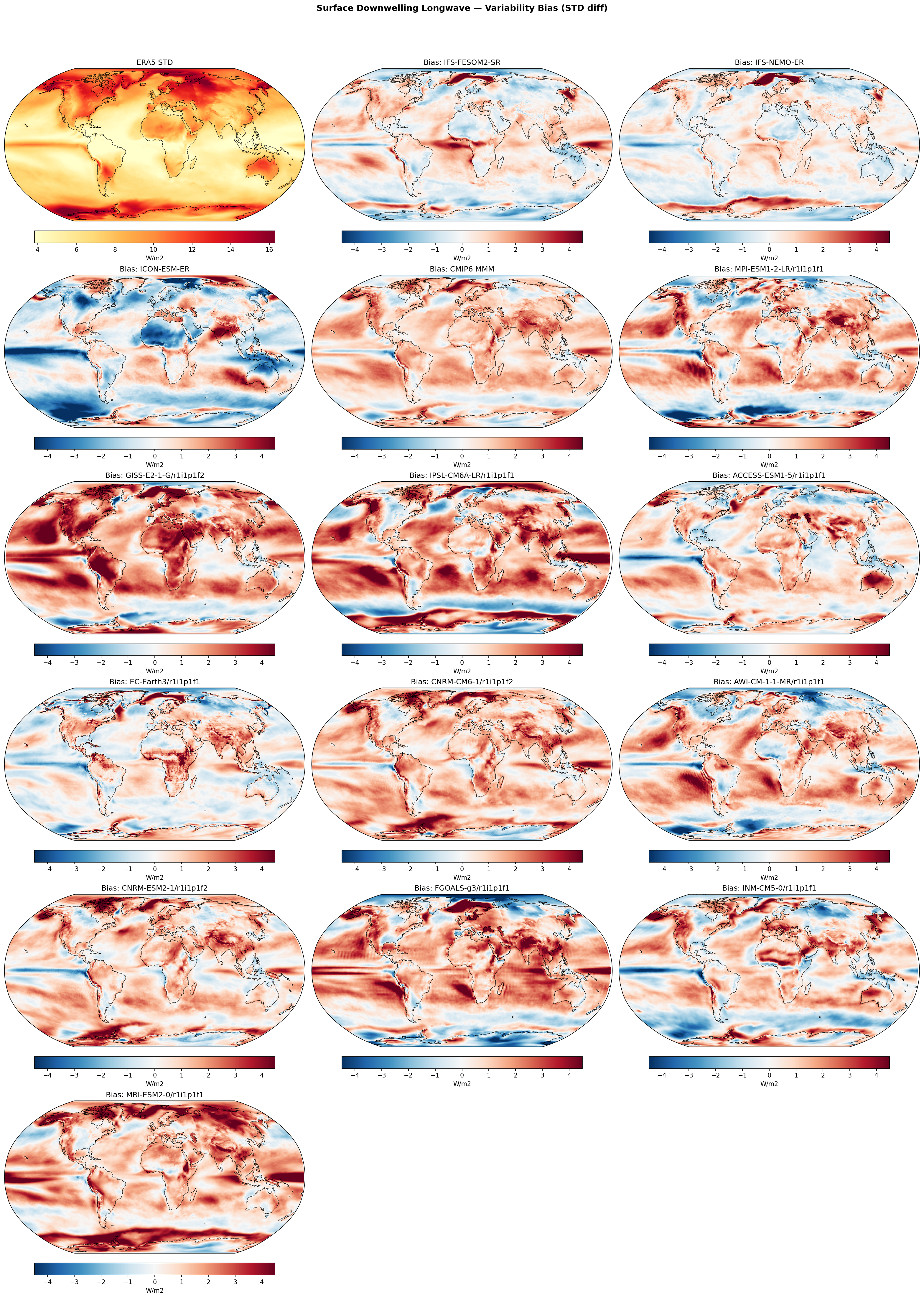
Summary high
This diagnostic evaluates the variability (standard deviation of anomalies) of surface downwelling longwave radiation. The high-resolution IFS models (IFS-NEMO-ER, IFS-FESOM2-SR) demonstrate superior agreement with ERA5 compared to the CMIP6 ensemble, which generally overestimates variability, whereas ICON-ESM-ER systematically underestimates it.
Key Findings
- IFS-NEMO-ER achieves the best agreement with observations (RMSE ~0.99 W/m²), showing only mild biases compared to the broader ensemble.
- Most CMIP6 models and the Multi-Model Mean (MMM) exhibit a strong positive bias (red), indicating they simulate significantly more temporal variability in downwelling longwave radiation than ERA5, particularly over land.
- ICON-ESM-ER stands out with a widespread negative bias (blue), underestimating variability globally (RMSE ~1.74 W/m²), especially in the tropics and Northern Hemisphere landmasses.
Spatial Patterns
In ERA5, peak variability occurs over Northern Hemisphere continents and the Southern Ocean. The CMIP6 ensemble exaggerates this pattern, showing intense positive variability biases over South America, Africa, and the tropical oceans. In contrast, ICON-ESM-ER shows dampened variability in the tropical Pacific (ENSO region) and across Eurasia. The IFS models show a mixed pattern with slight underestimation in the tropical Pacific and slight overestimation over NH land, but amplitudes are much smaller than in CMIP6.
Model Agreement
There is a distinct divergence between model groups: CMIP6 models generally overestimate variability (positive bias), ICON-ESM-ER underestimates it (negative bias), and the IFS-based EERIE models (NEMO/FESOM) fall in between, closest to ERA5. The IFS models agree well with each other, though IFS-FESOM2-SR is slightly more variable than IFS-NEMO-ER.
Physical Interpretation
Variability in surface downwelling longwave radiation is driven by fluctuations in lower tropospheric temperature, specific humidity, and cloud cover. The systematic positive bias in CMIP6 suggests excessive volatility in simulated cloud cover or stronger-than-observed land-atmosphere coupling. ICON's negative bias suggests overly persistent cloud decks or dampened synoptic/convective activity reducing the variance of temperature and moisture fields. The IFS models appear to capture the transition between clear and cloudy sky regimes more realistically.
Caveats
- ERA5 is a reanalysis product; while it assimilates temperature and humidity, radiative fluxes are model-derived and subject to the reanalysis model's own cloud physics biases.
- Biases in the tropical Pacific may be linked to how models represent ENSO amplitude, which strongly modulates local cloudiness and temperature.
Surface Downwelling Shortwave — Variability (STD)
| Variables | rsds |
|---|---|
| Models | IFS-FESOM2-SR, IFS-NEMO-ER, ICON-ESM-ER, CMIP6 MMM, MPI-ESM1-2-LR/r1i1p1f1, GISS-E2-1-G/r1i1p1f2, IPSL-CM6A-LR/r1i1p1f1, ACCESS-ESM1-5/r1i1p1f1, EC-Earth3/r1i1p1f1, CNRM-CM6-1/r1i1p1f2, AWI-CM-1-1-MR/r1i1p1f1, CNRM-ESM2-1/r1i1p1f2, FGOALS-g3/r1i1p1f1, INM-CM5-0/r1i1p1f1, MRI-ESM2-0/r1i1p1f1 |
| Reference Dataset | ERA5 |
| Units | W/m2 |
| Period | 1980–2014 |
| IFS-FESOM2-SR | Std Gmean: 12.40 · Diff Gmean: 0.49 · Rmse: 2.25 |
| IFS-NEMO-ER | Std Gmean: 12.30 · Diff Gmean: 0.40 · Rmse: 1.94 |
| ICON-ESM-ER | Std Gmean: 11.38 · Diff Gmean: -0.53 · Rmse: 3.33 |
| CMIP6 MMM | Std Gmean: 13.97 · Diff Gmean: 2.07 · Rmse: 2.88 |
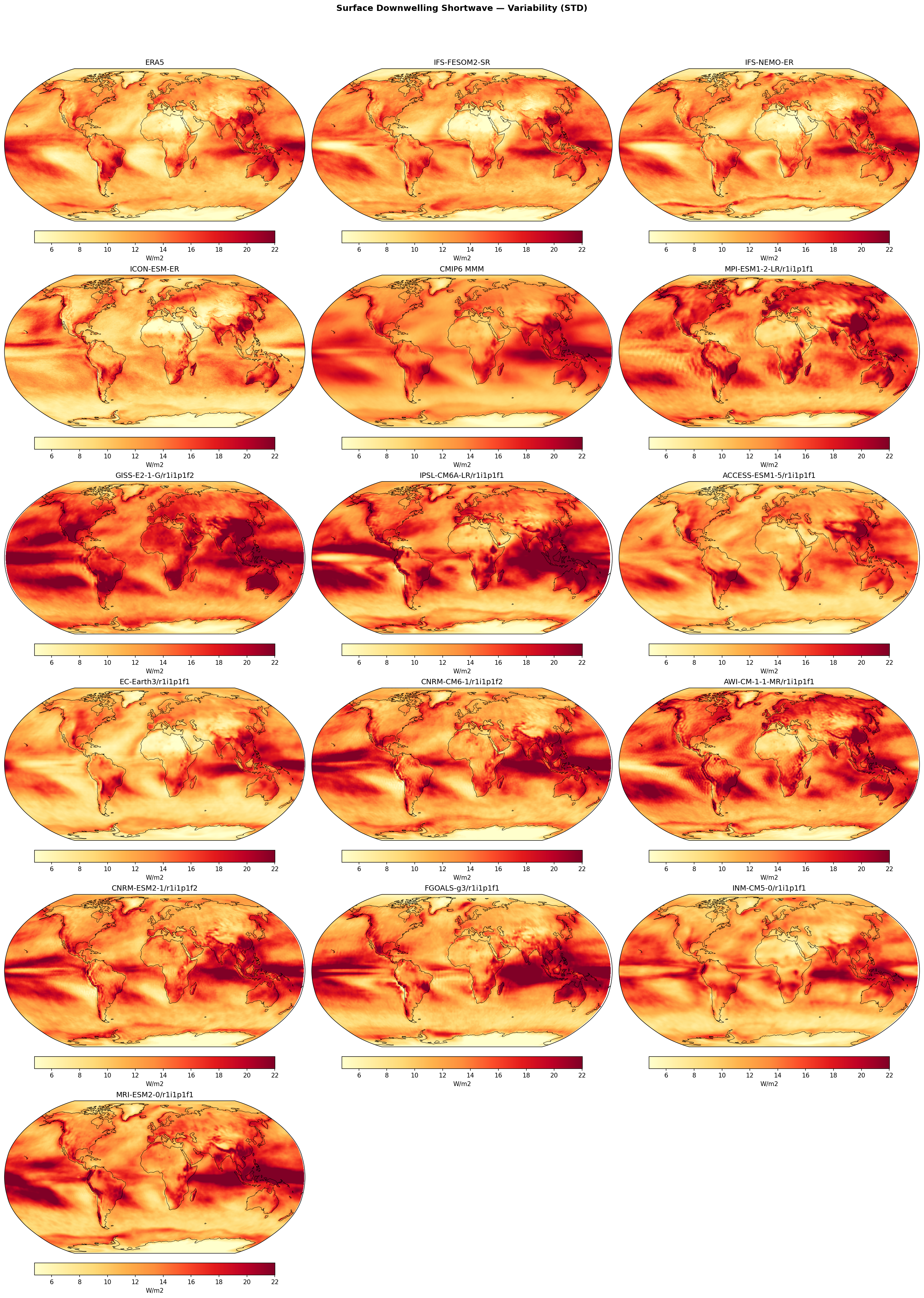
Summary high
This diagnostic evaluates the standard deviation of deseasonalised, detrended surface downwelling shortwave radiation (rsds), serving as a proxy for the temporal variability of cloud cover and radiative effects. The high-resolution IFS models demonstrate superior agreement with ERA5 reanalysis compared to the lower-resolution ICON-ESM-ER and the CMIP6 Multi-Model Mean.
Key Findings
- IFS-NEMO-ER and IFS-FESOM2-SR show excellent agreement with ERA5, exhibiting the lowest RMSEs (1.94 and 2.25 W/m² respectively) and accurately capturing the spatial structure of variability in the ENSO region and storm tracks.
- ICON-ESM-ER systematically underestimates surface shortwave variability globally (global mean difference -0.53 W/m²), appearing visually 'washed out' with notably suppressed variability in the tropical Pacific and mid-latitude storm tracks relative to ERA5.
- The CMIP6 Multi-Model Mean (MMM) significantly overestimates variability (global mean difference +2.07 W/m²), particularly in the Southern Ocean and tropical convergence zones, suggesting that coarser conventional models may exhibit excessive 'flickering' or instability in cloud radiative effects.
Spatial Patterns
High variability (dark red, >16 W/m²) is observed in the tropical Pacific (driven by ENSO dynamics), the Indo-Pacific Warm Pool, and mid-latitude storm tracks where frontal cloud systems dominate. The IFS models correctly resolve the confined 'tongue' of variability associated with ENSO, whereas the CMIP6 MMM smears this feature zonally and meridionally. ICON-ESM-ER shows reduced contrast between active convective regions and stable subtropical highs.
Model Agreement
The two IFS variants (NEMO and FESOM) align closely with ERA5, outperforming both the CMIP6 ensemble and ICON. There is a large spread among individual CMIP6 models, with some (e.g., GISS-E2-1-G, MRI-ESM2-0) showing extreme variability (>20 W/m² widespread) and others (e.g., INM-CM5-0) showing lower variability similar to ICON.
Physical Interpretation
Since solar output is relatively constant on these timescales, rsds variability is primarily driven by cloud cover fluctuations (cloud fraction and optical depth). The high variability in the tropical Pacific reflects ENSO-related shifts in convection. The underestimation by ICON suggests a model climatology with too-persistent cloud features or dampened convective variability. Conversely, the high variability in CMIP6 models may stem from parameterized convection schemes triggering too frequently or shifting location too readily (e.g., double ITCZ flickering).
Caveats
- ERA5 rsds is a model-derived product (reanalysis) rather than direct observation, though it assimilates vast amounts of atmospheric data.
- High variability in specific CMIP6 models (e.g., GISS) dominates the MMM appearance, potentially skewing the visual comparison against the more coherent high-res models.
Surface Downwelling Shortwave — Variability Bias (STD diff)
| Variables | rsds |
|---|---|
| Models | IFS-FESOM2-SR, IFS-NEMO-ER, ICON-ESM-ER, CMIP6 MMM, MPI-ESM1-2-LR/r1i1p1f1, GISS-E2-1-G/r1i1p1f2, IPSL-CM6A-LR/r1i1p1f1, ACCESS-ESM1-5/r1i1p1f1, EC-Earth3/r1i1p1f1, CNRM-CM6-1/r1i1p1f2, AWI-CM-1-1-MR/r1i1p1f1, CNRM-ESM2-1/r1i1p1f2, FGOALS-g3/r1i1p1f1, INM-CM5-0/r1i1p1f1, MRI-ESM2-0/r1i1p1f1 |
| Reference Dataset | ERA5 |
| Units | W/m2 |
| Period | 1980–2014 |
| IFS-FESOM2-SR | Std Gmean: 12.40 · Diff Gmean: 0.49 · Rmse: 2.25 |
| IFS-NEMO-ER | Std Gmean: 12.30 · Diff Gmean: 0.40 · Rmse: 1.94 |
| ICON-ESM-ER | Std Gmean: 11.38 · Diff Gmean: -0.53 · Rmse: 3.33 |
| CMIP6 MMM | Std Gmean: 13.97 · Diff Gmean: 2.07 · Rmse: 2.88 |
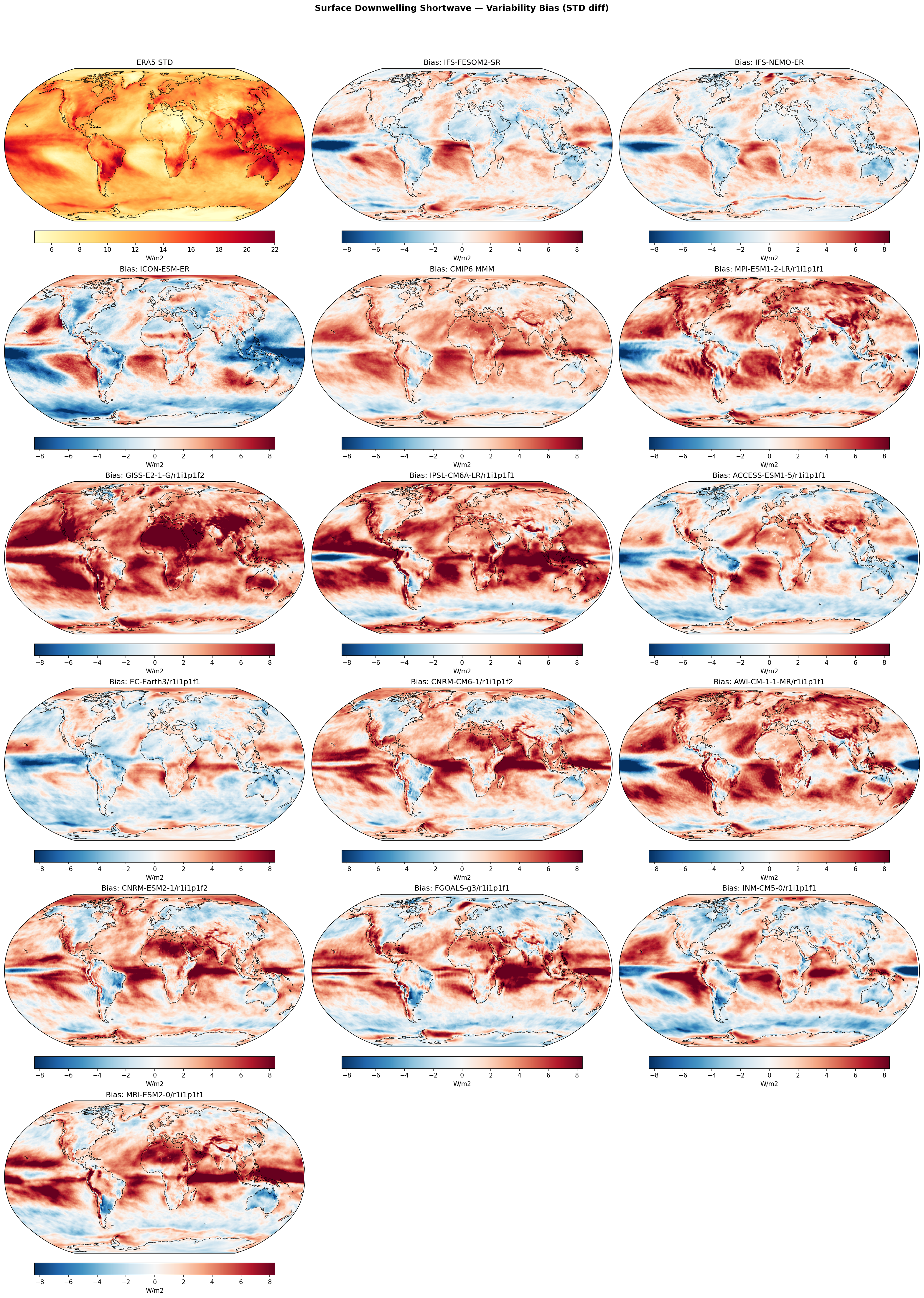
Summary high
This diagnostic evaluates the variability (standard deviation of anomalies) of surface downwelling shortwave radiation. The high-resolution IFS models (NEMO/FESOM) show the closest agreement with ERA5, whereas the CMIP6 Multi-Model Mean and most legacy models systematically overestimate variability, and ICON-ESM-ER systematically underestimates it.
Key Findings
- IFS-NEMO-ER and IFS-FESOM2-SR perform best, exhibiting the lowest RMSE (~1.9–2.2 W/m²) and weakest bias magnitudes, though they slightly underestimate variability in the tropical ITCZ/SPCZ regions.
- The CMIP6 Multi-Model Mean and several individual models (e.g., GISS-E2-1-G, MRI-ESM2-0) show a strong, widespread positive bias, indicating they simulate excessive temporal variability in surface solar radiation (global mean diff +2.1 W/m²).
- ICON-ESM-ER is distinct from the other high-resolution models, showing a widespread negative bias (too little variability), particularly over the tropical oceans and Southern Ocean.
- A distinct spatial pattern appears in the IFS models: negative bias (too stable) in the deep tropical convective zones, contrasted with positive bias (too variable) in the mid-latitude storm tracks.
Spatial Patterns
In ERA5, highest variability (>18 W/m²) is found in the Tropical Warm Pool and monsoon regions, driven by convective cloud dynamics. The IFS models capture the spatial structure well but dampen the amplitude in the central Pacific. CMIP6 models tend to exaggerate variability over the entire tropical band and Southern Ocean. ICON-ESM-ER suppresses variability broadly across the global ocean.
Model Agreement
The two IFS variants (FESOM/NEMO) agree strongly with each other. There is significant divergence between the high-resolution models (IFS vs ICON) and between the high-resolution group and the CMIP6 ensemble. CMIP6 models are generally 'noisier' than ERA5, while ICON is 'quieter'.
Physical Interpretation
Variability in surface shortwave radiation is primarily controlled by cloud intermittency and optical depth fluctuations. The positive bias in CMIP6 suggests 'flickering' cloud behavior or binary convective triggering (on/off) that lacks the persistence seen in nature. The negative bias in ICON suggests clouds are too persistent or spatially uniform. The IFS dipole (stable tropics, variable mid-latitudes) may reflect differing performance of convective parameterizations vs. large-scale cloud schemes.
Caveats
- ERA5 is a reanalysis product and relies on its own cloud parameterizations, which introduces some uncertainty as a 'truth' baseline for radiative variables.
- The analysis does not distinguish between cloud cover fraction variability and cloud optical depth variability.
2m Temperature — Variability (STD)
| Variables | tas |
|---|---|
| Models | IFS-FESOM2-SR, IFS-NEMO-ER, ICON-ESM-ER, CMIP6 MMM |
| Reference Dataset | ERA5 |
| Units | K |
| Period | 1980–2014 |
| IFS-FESOM2-SR | Std Gmean: 1.04 · Diff Gmean: 0.06 · Rmse: 0.21 |
| IFS-NEMO-ER | Std Gmean: 1.02 · Diff Gmean: 0.05 · Rmse: 0.22 |
| ICON-ESM-ER | Std Gmean: 0.95 · Diff Gmean: -0.02 · Rmse: 0.28 |
| CMIP6 MMM | Std Gmean: 1.05 · Diff Gmean: 0.08 · Rmse: 0.18 |
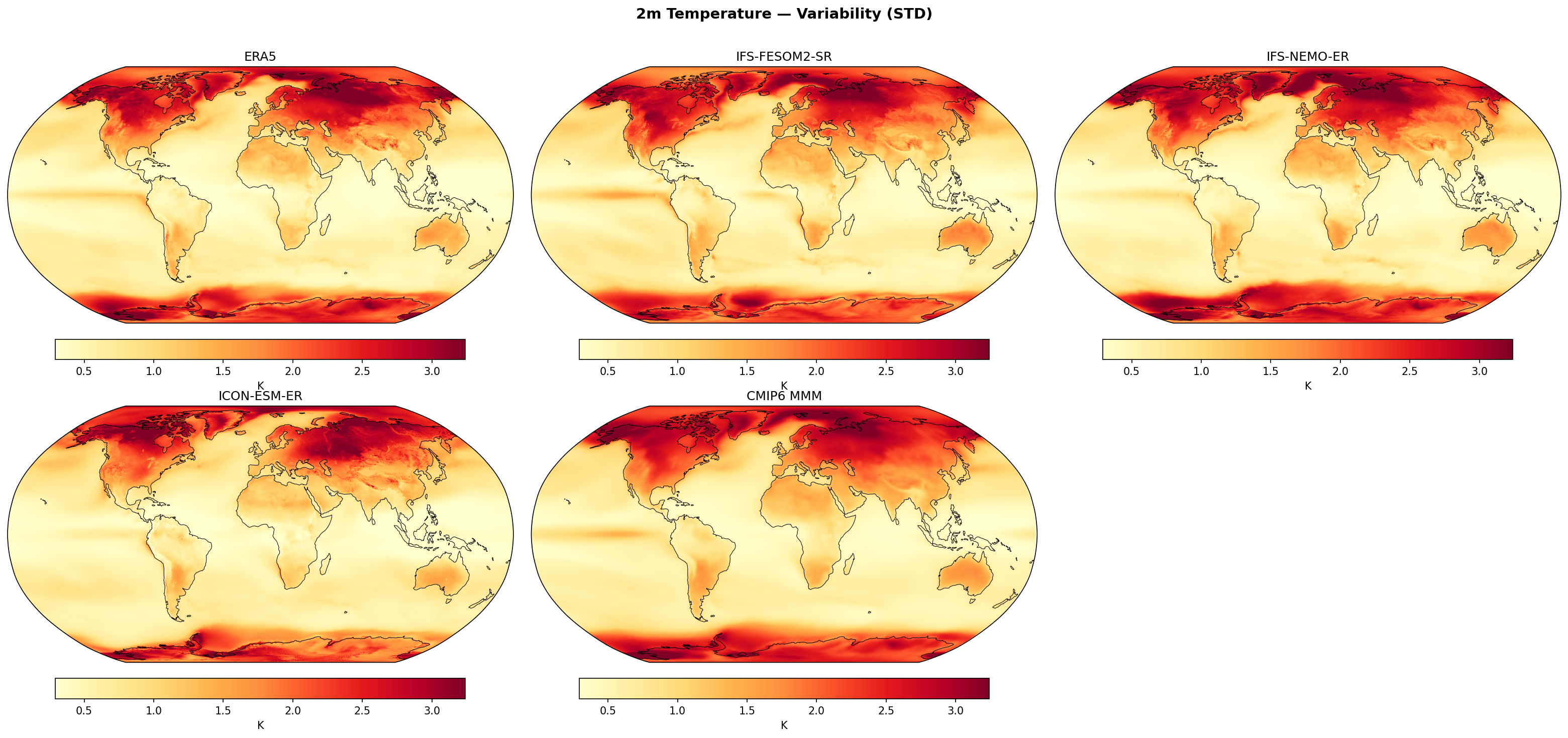
Summary high
This figure compares the standard deviation of monthly 2m temperature anomalies (internal variability) in high-resolution EERIE models against ERA5 and CMIP6. The models successfully reproduce the dominant global patterns, including high variability over Northern Hemisphere continents and sea-ice margins, though IFS models slightly overestimate and ICON underestimates the global mean variability.
Key Findings
- All models capture the primary variability hotspots: high-latitude continental interiors (Siberia, North America), sea-ice marginal zones (Arctic, Southern Ocean), and the ENSO region.
- IFS-FESOM2-SR and IFS-NEMO-ER show very similar performance, both slightly overestimating global mean variability (~+0.05-0.06 K bias) but aligning well with ERA5 spatial structures.
- ICON-ESM-ER generally underestimates variability (bias -0.025 K) and exhibits a noticeably weaker ENSO signature in the tropical Pacific compared to ERA5 and the IFS models.
- CMIP6 MMM has the lowest RMSE (0.176 K), indicating that the multi-model ensemble average captures the spatial distribution of variability robustly, despite lacking the fine-scale details of the high-resolution simulations.
Spatial Patterns
Variability is highest (>3 K) over Northern Hemisphere land masses (due to low heat capacity) and polar sea-ice margins (due to ice edge movement). A distinct tongue of variability (~1.5-2 K) extends westward from South America along the equator, corresponding to ENSO. The Southern Ocean shows a zonal band of high variability driven by sea-ice dynamics.
Model Agreement
There is strong inter-model agreement on the location of high-variability regions. The IFS models track ERA5 intensity closely, particularly in the ENSO region and Northern Hemisphere land. ICON is the outlier with dampened variability, particularly visible in the narrower and weaker ENSO tongue.
Physical Interpretation
The patterns reflect fundamental physical drivers: low thermal inertia of land surfaces leads to higher variability than oceans; sea-ice variation creates large surface temperature anomalies at the ice edge; and ENSO dynamics drive interannual variability in the tropical Pacific. The muted signal in ICON suggests either dampened ENSO dynamics or stronger damping feedbacks in that model formulation.
Caveats
- The analysis is based on standard deviation of detrended data; it does not distinguish between timescales (e.g., interannual vs. decadal).
- ICON's lower variability might be influenced by its specific tuning or resolution-dependent effective diffusivity.
2m Temperature — Variability Bias (STD diff)
| Variables | tas |
|---|---|
| Models | IFS-FESOM2-SR, IFS-NEMO-ER, ICON-ESM-ER, CMIP6 MMM |
| Reference Dataset | ERA5 |
| Units | K |
| Period | 1980–2014 |
| IFS-FESOM2-SR | Std Gmean: 1.04 · Diff Gmean: 0.06 · Rmse: 0.21 |
| IFS-NEMO-ER | Std Gmean: 1.02 · Diff Gmean: 0.05 · Rmse: 0.22 |
| ICON-ESM-ER | Std Gmean: 0.95 · Diff Gmean: -0.02 · Rmse: 0.28 |
| CMIP6 MMM | Std Gmean: 1.05 · Diff Gmean: 0.08 · Rmse: 0.18 |
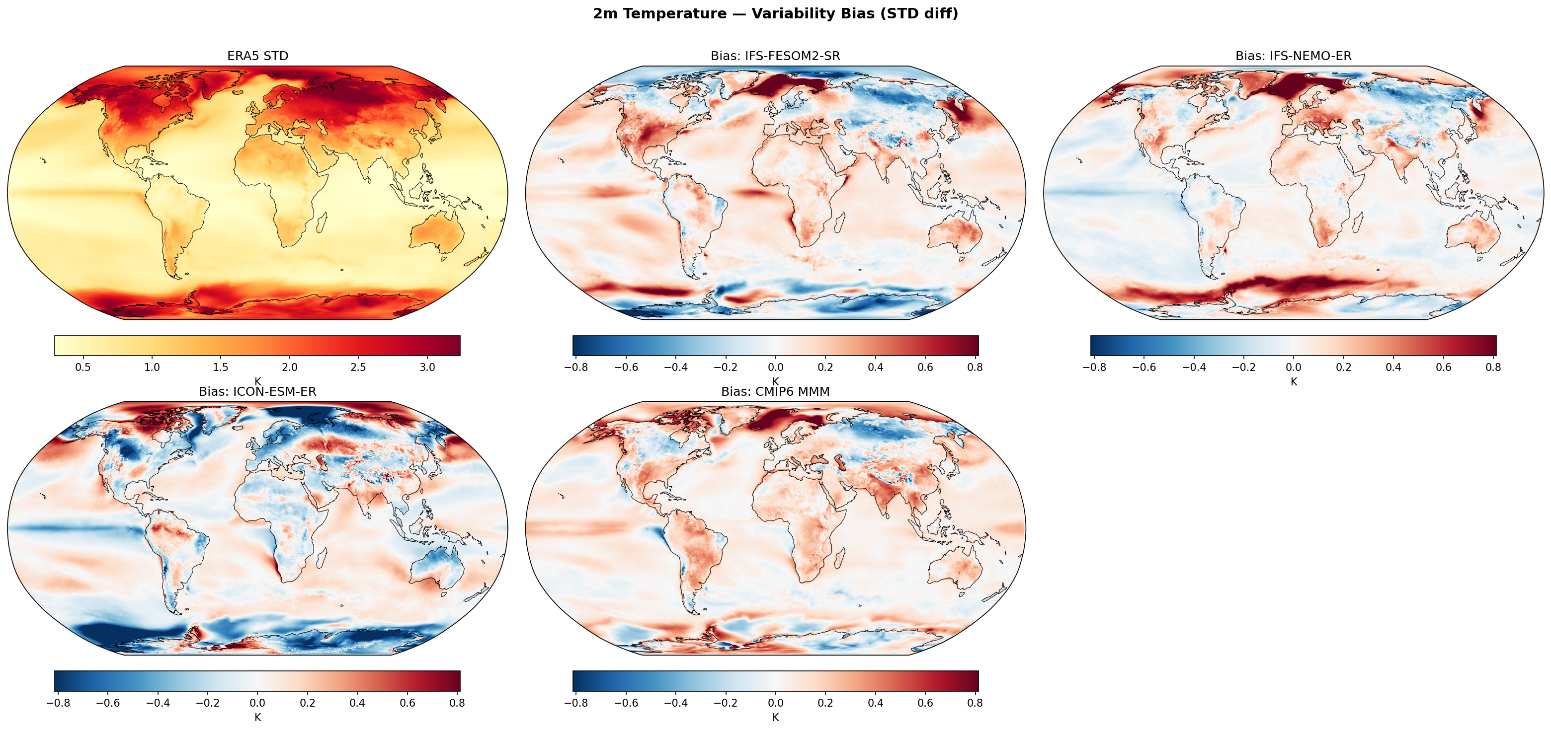
Summary high
This figure evaluates the variability (standard deviation of anomalies) of 2m temperature in three high-resolution models and the CMIP6 multi-model mean against ERA5 reanalysis. The analysis reveals significant discrepancies in the representation of variability in the Southern Ocean sea-ice zone, the tropical Pacific (ENSO), and Northern Hemisphere landmasses.
Key Findings
- IFS-NEMO-ER exhibits a distinct, intense ring of excessive variability (>0.8 K bias) surrounding Antarctica, likely linked to the marginal sea ice zone dynamics, which contrasts sharply with the negative bias seen in IFS-FESOM2-SR in the same region.
- IFS-FESOM2-SR and the CMIP6 MMM overestimate variability in the tropical Pacific, suggesting an overly active or spatially extensive ENSO mode, whereas ICON-ESM-ER and IFS-NEMO-ER are closer to observations in this region.
- ICON-ESM-ER generally underestimates temperature variability globally (mean bias -0.02 K), with notable deficits over Northern Hemisphere continents (North America, Siberia) and the Arctic, resulting in the highest RMSE (0.28 K) among the groups shown.
Spatial Patterns
ERA5 shows peak variability over high-latitude landmasses and the sea ice edges. Model biases are regionally concentrated: IFS-FESOM2-SR is dominated by positive biases in the tropics and subtropics; IFS-NEMO-ER is dominated by the positive Southern Ocean zonal band; ICON-ESM-ER shows widespread negative biases over ocean and NH land, with complex mixed signals in the polar regions.
Model Agreement
The two IFS-based models share some atmospheric characteristics but diverge strongly in the Southern Ocean, highlighting the impact of the ocean-ice component (NEMO vs. FESOM). The CMIP6 MMM achieves the lowest RMSE (0.18 K) due to ensemble smoothing but shares the tropical positive bias seen in IFS-FESOM2-SR.
Physical Interpretation
The high variability bias in the Southern Ocean for IFS-NEMO-ER likely stems from excessive fluctuation in sea ice extent or concentration, where the alternation between open water and ice creates large temperature variances. The positive tropical Pacific bias in IFS-FESOM2-SR indicates enhanced ENSO amplitude. The underestimation of variability over land in ICON-ESM-ER suggests overly damped land-atmosphere coupling or boundary layer processes.
Caveats
- The CMIP6 MMM naturally has reduced variability due to averaging inconsistent internal variability phases across models, yet it still shows a positive mean bias.
- The analysis does not distinguish between interannual (e.g., ENSO) and sub-seasonal variability, both of which contribute to the calculated standard deviation.
10m U Wind — Variability (STD)
| Variables | uas |
|---|---|
| Models | IFS-FESOM2-SR, IFS-NEMO-ER, ICON-ESM-ER, CMIP6 MMM, MPI-ESM1-2-LR/r1i1p1f1, GISS-E2-1-G/r1i1p1f2, IPSL-CM6A-LR/r1i1p1f1, ACCESS-ESM1-5/r1i1p1f1, EC-Earth3/r1i1p1f1, CNRM-CM6-1/r1i1p1f2, AWI-CM-1-1-MR/r1i1p1f1, CNRM-ESM2-1/r1i1p1f2, INM-CM5-0/r1i1p1f1, MRI-ESM2-0/r1i1p1f1 |
| Reference Dataset | ERA5 |
| Units | m/s |
| Period | 1980–2014 |
| IFS-FESOM2-SR | Std Gmean: 1.22 · Diff Gmean: 0.03 · Rmse: 0.19 |
| IFS-NEMO-ER | Std Gmean: 1.20 · Diff Gmean: -0.00 · Rmse: 0.15 |
| ICON-ESM-ER | Std Gmean: 1.21 · Diff Gmean: 0.02 · Rmse: 0.29 |
| CMIP6 MMM | Std Gmean: 1.27 · Diff Gmean: 0.08 · Rmse: 0.19 |
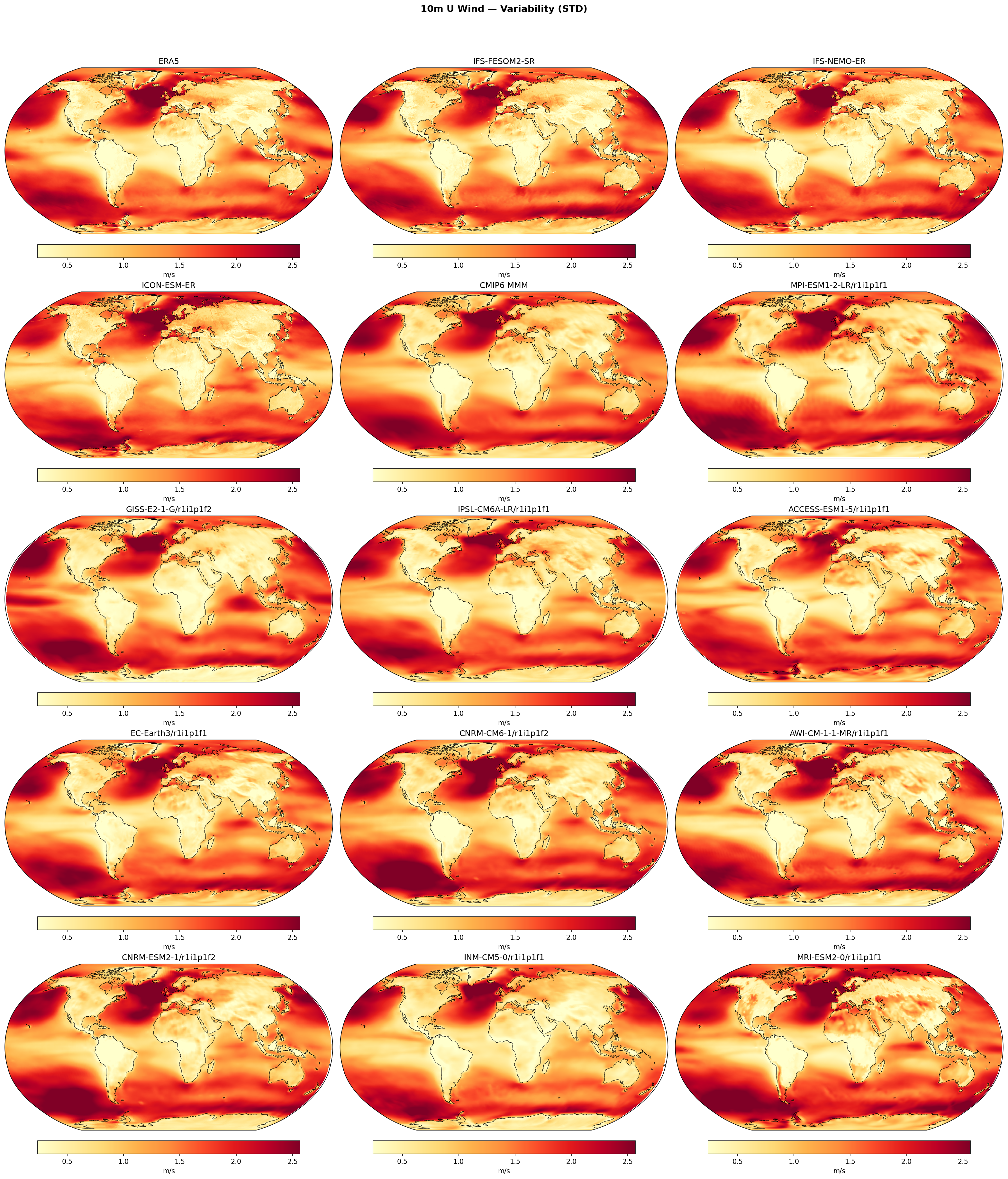
Summary high
This multi-panel figure compares the standard deviation of deseasonalised, detrended monthly 10m zonal wind (U-wind) across high-resolution EERIE models, CMIP6 models, and ERA5 reanalysis. The high-resolution IFS models (NEMO and FESOM2) demonstrate superior skill in reproducing observed variability patterns, particularly in the mid-latitude storm tracks, compared to the broader spread found in the CMIP6 ensemble.
Key Findings
- Variability is dominated by the major storm tracks in the North Atlantic, North Pacific, and Southern Ocean, where STD exceeds 2.0 m/s.
- IFS-NEMO-ER shows exceptional agreement with ERA5, with a near-zero global mean bias (-0.0005 m/s) and the lowest RMSE (0.145 m/s) of the highlighted models.
- The CMIP6 Multi-Model Mean (MMM) tends to overestimate global variability (+0.078 m/s bias) and individual CMIP6 models show large dispersion, with INM-CM5-0 significantly underestimating storm track intensity.
- ICON-ESM-ER exhibits higher RMSE (0.286 m/s) than the IFS variants, suggesting some spatial displacement or structural differences in variability despite reasonable global mean magnitude.
Spatial Patterns
Maximum variability is zonally oriented along the oceanic storm tracks at 40-60° latitude in both hemispheres. The Southern Ocean exhibits a continuous band of high variability (>2.5 m/s), while Northern Hemisphere patterns are more basin-localized (N. Atlantic and N. Pacific). Tropical variability is generally lower (<1 m/s) but shows structure in the Pacific related to ENSO dynamics. Variability over land is consistently lower than over oceans due to surface friction.
Model Agreement
IFS-NEMO-ER and IFS-FESOM2-SR show very strong spatial agreement with ERA5, capturing the sharpness and intensity of storm tracks accurately. In contrast, CMIP6 models vary widely: models like ACCESS-ESM1-5 and MRI-ESM2-0 show vigorous variability similar to ERA5, while GISS-E2-1-G and INM-CM5-0 show noticeably muted variability in the Southern Ocean. ICON-ESM-ER captures the general patterns but appears to have slightly different spatial structures in the high latitudes compared to IFS and ERA5.
Physical Interpretation
The patterns reflect synoptic-scale baroclinic instability (cyclone/anticyclone passage) in the mid-latitudes and interannual variability (e.g., ENSO) in the tropics. The higher resolution of the IFS-SR/ER models (~10 km) allows for a better representation of sharp frontal gradients and storm intensity compared to coarser CMIP6 models (~100 km), which may smooth out these transient features. The lower variability in models like INM-CM5-0 is a known characteristic often linked to their specific diffusive parameterizations.
Caveats
- Data is deseasonalised, so the variability represents interannual and sub-seasonal (monthly) anomalies, not the seasonal cycle amplitude.
- Differences in land surface roughness parameterizations may contribute to variability discrepancies over continents.
10m U Wind — Variability Bias (STD diff)
| Variables | uas |
|---|---|
| Models | IFS-FESOM2-SR, IFS-NEMO-ER, ICON-ESM-ER, CMIP6 MMM, MPI-ESM1-2-LR/r1i1p1f1, GISS-E2-1-G/r1i1p1f2, IPSL-CM6A-LR/r1i1p1f1, ACCESS-ESM1-5/r1i1p1f1, EC-Earth3/r1i1p1f1, CNRM-CM6-1/r1i1p1f2, AWI-CM-1-1-MR/r1i1p1f1, CNRM-ESM2-1/r1i1p1f2, INM-CM5-0/r1i1p1f1, MRI-ESM2-0/r1i1p1f1 |
| Reference Dataset | ERA5 |
| Units | m/s |
| Period | 1980–2014 |
| IFS-FESOM2-SR | Std Gmean: 1.22 · Diff Gmean: 0.03 · Rmse: 0.19 |
| IFS-NEMO-ER | Std Gmean: 1.20 · Diff Gmean: -0.00 · Rmse: 0.15 |
| ICON-ESM-ER | Std Gmean: 1.21 · Diff Gmean: 0.02 · Rmse: 0.29 |
| CMIP6 MMM | Std Gmean: 1.27 · Diff Gmean: 0.08 · Rmse: 0.19 |
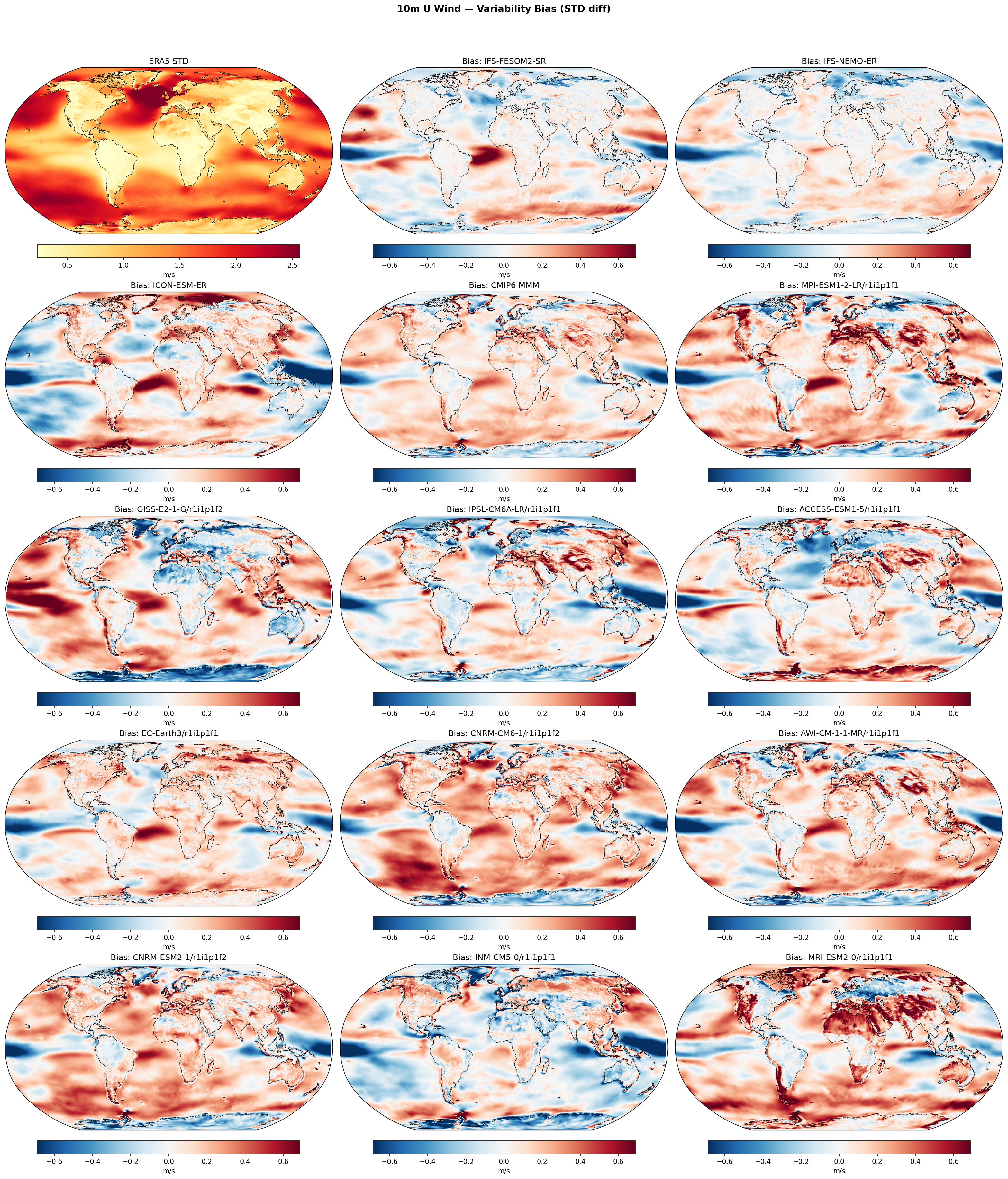
Summary high
This diagnostic evaluates the variability (standard deviation) of 10m zonal wind (U component), comparing high-resolution EERIE models and CMIP6 simulations against ERA5 reanalysis. The high-resolution IFS-NEMO-ER model demonstrates the best agreement with observations, while ICON-ESM-ER significantly underestimates variability in key regions.
Key Findings
- IFS-NEMO-ER achieves the lowest RMSE (0.145 m/s) and near-zero global mean bias, showing excellent capture of wind variability patterns compared to other models.
- ICON-ESM-ER exhibits distinct negative variability biases (blue) in the Southern Ocean storm track and tropical convergence zones, indicating suppressed synoptic or convective activity relative to ERA5.
- Many coarse-resolution CMIP6 models (e.g., MRI-ESM2-0, GISS-E2-1-G) show strong positive variability biases (red) over land and tropical oceans, suggesting issues with topographic drag or convective parameterisations.
- IFS-FESOM2-SR and IFS-NEMO-ER share a specific bias pattern in the tropical Pacific: overestimated variability in the central/western part and underestimated variability in the eastern cold tongue.
Spatial Patterns
ERA5 shows peak wind variability in the North Atlantic, North Pacific, and Southern Ocean storm tracks. Biases are spatially coherent: CMIP6 models tend to be too variable over continents (especially mountain ranges like the Andes and Himalayas) and tropical convective zones. The EERIE IFS models are relatively unbiased over extratropical oceans but show zonal asymmetry in the tropical Pacific. ICON-ESM-ER stands out with widespread low-variability bias in the Southern Hemisphere westerlies and ITCZ.
Model Agreement
There is significant divergence. IFS-NEMO-ER and IFS-FESOM2-SR agree relatively well with observations (low RMSE), whereas ICON-ESM-ER diverges with a high RMSE (0.286 m/s), worse than the CMIP6 Multi-Model Mean (0.193 m/s). CMIP6 individual members show high spread, with some (MPI-ESM1-2-LR) resembling the MMM and others (MRI-ESM2-0) showing extreme positive biases.
Physical Interpretation
The positive biases over land and tropics in coarser models likely result from 'grid-point storms'—intense, localized convective events or unresolved topographic interactions. The negative bias in ICON-ESM-ER's Southern Ocean suggests too zonal or stable flow with insufficient cyclonic activity. The tropical Pacific dipole in IFS models may relate to the representation of the Walker circulation and ENSO-related wind variability.
Caveats
- The STD metric aggregates all timescales (synoptic to interannual), so biases could stem from weather noise or ENSO amplitude differences.
- ERA5 reanalysis itself relies on model physics in data-sparse regions like the Southern Ocean, potentially influencing the 'observed' variability baseline.
10m V Wind — Variability (STD)
| Variables | vas |
|---|---|
| Models | IFS-FESOM2-SR, IFS-NEMO-ER, ICON-ESM-ER, CMIP6 MMM, MPI-ESM1-2-LR/r1i1p1f1, GISS-E2-1-G/r1i1p1f2, IPSL-CM6A-LR/r1i1p1f1, ACCESS-ESM1-5/r1i1p1f1, EC-Earth3/r1i1p1f1, CNRM-CM6-1/r1i1p1f2, AWI-CM-1-1-MR/r1i1p1f1, CNRM-ESM2-1/r1i1p1f2, INM-CM5-0/r1i1p1f1, MRI-ESM2-0/r1i1p1f1 |
| Reference Dataset | ERA5 |
| Units | m/s |
| Period | 1980–2014 |
| IFS-FESOM2-SR | Std Gmean: 0.95 · Diff Gmean: 0.02 · Rmse: 0.12 |
| IFS-NEMO-ER | Std Gmean: 0.94 · Diff Gmean: 0.00 · Rmse: 0.10 |
| ICON-ESM-ER | Std Gmean: 0.99 · Diff Gmean: 0.05 · Rmse: 0.19 |
| CMIP6 MMM | Std Gmean: 1.01 · Diff Gmean: 0.07 · Rmse: 0.15 |
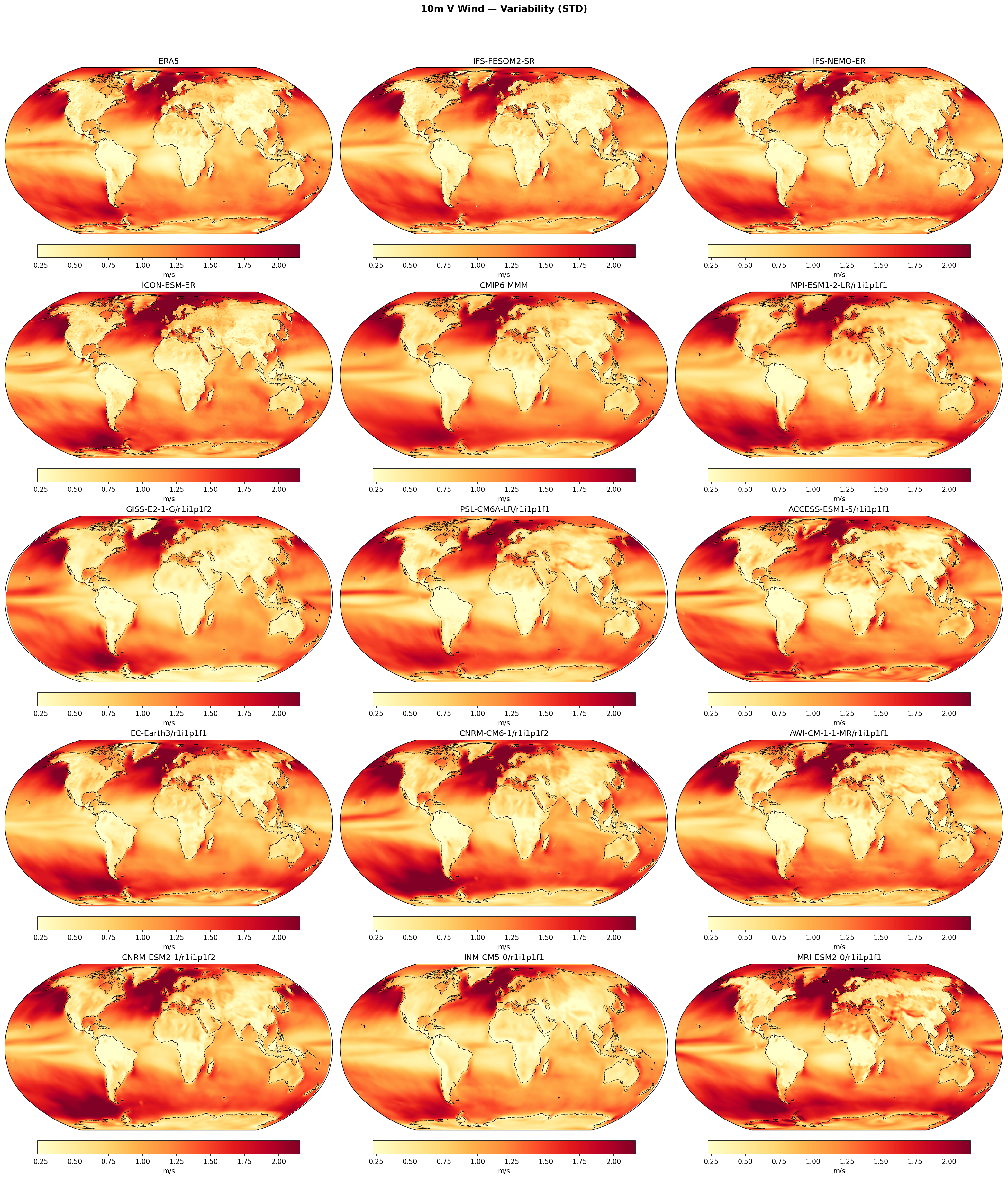
Summary high
This figure compares the standard deviation of monthly 10m meridional wind (V wind) variability across high-resolution EERIE models, the CMIP6 ensemble, and ERA5 reanalysis. The high-resolution IFS models (NEMO-ER and FESOM2-SR) demonstrate superior agreement with observations compared to ICON-ESM-ER and the CMIP6 Multi-Model Mean.
Key Findings
- IFS-NEMO-ER exhibits the best performance, with the lowest RMSE (0.10 m/s) and a negligible global mean bias (+0.003 m/s) relative to ERA5.
- ICON-ESM-ER overestimates variability generally, with a global positive bias (+0.054 m/s) and the highest RMSE (0.19 m/s) among the summary statistics provided, showing particularly intense signals in the Southern Ocean.
- The CMIP6 Multi-Model Mean shows a positive bias (+0.07 m/s) and reduced RMSE (0.15 m/s) compared to ICON, but visually lacks the sharp spatial definition of the storm tracks seen in the high-resolution IFS simulations.
- Individual CMIP6 models show a large spread in variability intensity; for example, ACCESS-ESM1-5 is highly energetic in the Southern Ocean, while INM-CM5-0 is notably damped.
Spatial Patterns
Dominant features include high variability (>1.75 m/s) in the Southern Ocean, North Atlantic, and North Pacific storm tracks, consistent with synoptic eddy activity. The ITCZ and SPCZ regions in the tropics also show elevated variability. Land areas exhibit lower variability due to surface roughness, though orographic features modify this locally.
Model Agreement
The two IFS-based EERIE models agree very closely with ERA5 in both magnitude and spatial distribution. ICON-ESM-ER captures the correct patterns but with excessive amplitude. The CMIP6 ensemble displays significant inter-model spread, particularly in the Southern Ocean and tropics.
Physical Interpretation
Meridional wind variability at monthly scales traces the tracks of extratropical cyclones and the meandering of jet streams (e.g., storm tracks). High-resolution models (IFS-NEMO-ER, IFS-FESOM2-SR) likely resolve air-sea coupling and synoptic pressure gradients more accurately than coarser models, leading to variability statistics that closer match reanalysis.
Caveats
- Analysis is based on monthly means, which smooths out high-frequency synoptic extremes; this metric reflects the low-frequency variability of the storm tracks rather than instantaneous storm intensity.
- RMSE values suggest ICON-ESM-ER has larger local errors despite a lower global mean bias than the CMIP6 MMM.
10m V Wind — Variability Bias (STD diff)
| Variables | vas |
|---|---|
| Models | IFS-FESOM2-SR, IFS-NEMO-ER, ICON-ESM-ER, CMIP6 MMM, MPI-ESM1-2-LR/r1i1p1f1, GISS-E2-1-G/r1i1p1f2, IPSL-CM6A-LR/r1i1p1f1, ACCESS-ESM1-5/r1i1p1f1, EC-Earth3/r1i1p1f1, CNRM-CM6-1/r1i1p1f2, AWI-CM-1-1-MR/r1i1p1f1, CNRM-ESM2-1/r1i1p1f2, INM-CM5-0/r1i1p1f1, MRI-ESM2-0/r1i1p1f1 |
| Reference Dataset | ERA5 |
| Units | m/s |
| Period | 1980–2014 |
| IFS-FESOM2-SR | Std Gmean: 0.95 · Diff Gmean: 0.02 · Rmse: 0.12 |
| IFS-NEMO-ER | Std Gmean: 0.94 · Diff Gmean: 0.00 · Rmse: 0.10 |
| ICON-ESM-ER | Std Gmean: 0.99 · Diff Gmean: 0.05 · Rmse: 0.19 |
| CMIP6 MMM | Std Gmean: 1.01 · Diff Gmean: 0.07 · Rmse: 0.15 |
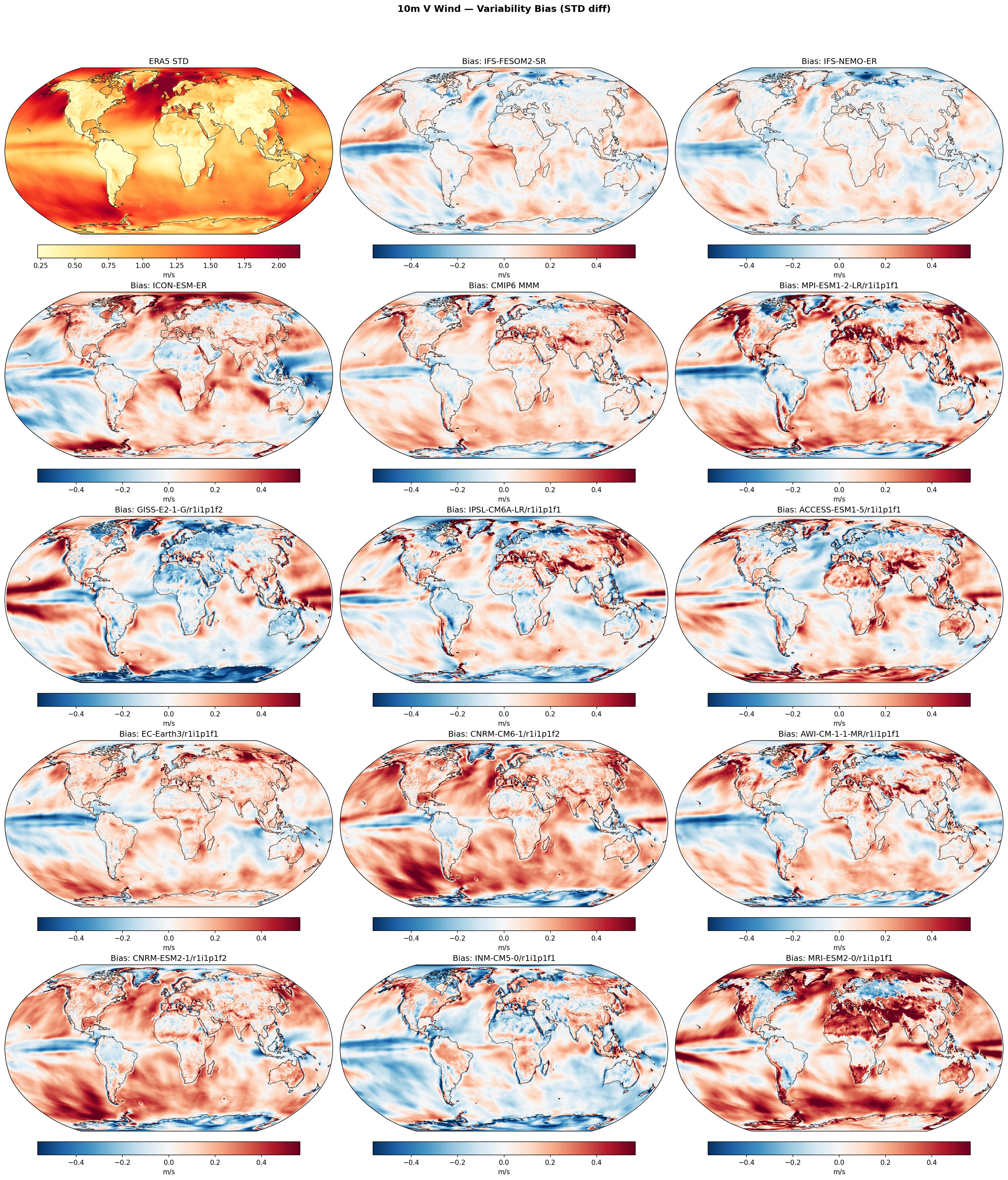
Summary high
This diagnostic evaluates the variability (standard deviation) of 10m meridional wind (V component) in high-resolution EERIE models compared to ERA5 and the CMIP6 ensemble. The IFS-based high-resolution models demonstrate superior skill with minimal biases, while ICON-ESM-ER and CMIP6 models exhibit larger, regionally distinct errors.
Key Findings
- IFS-NEMO-ER and IFS-FESOM2-SR show excellent agreement with ERA5, achieving the lowest global RMSEs (0.10 m/s and 0.12 m/s respectively) and avoiding the widespread biases seen in other models.
- CMIP6 models consistently overestimate wind variability over land surfaces and in the subtropics (positive bias), a systematic error that is largely absent in the high-resolution EERIE simulations.
- ICON-ESM-ER performs poorly relative to the other high-resolution models and even the CMIP6 MMM (RMSE 0.19 m/s vs 0.15 m/s), driven by excessive variability in the Southern Ocean and pronounced zonal biases in the tropics.
Spatial Patterns
ERA5 shows peak V-wind variability in the storm tracks and ITCZ. CMIP6 models exhibit a 'red' positive bias over most continents, suggesting insufficient frictional damping or topographic blocking. ICON-ESM-ER displays a distinct dipole bias in the tropics and strong positive anomalies in the Southern Ocean storm track. The IFS models show a slight negative bias (underestimation) in the tropical Pacific ITCZ region but are otherwise neutral.
Model Agreement
There is a strong divergence in performance: IFS models align closely with observations, whereas ICON-ESM-ER and individual CMIP6 models show large discrepancies. The CMIP6 MMM masks some individual model errors but retains a systematic land-bias. ICON deviates significantly from the IFS models in the Southern Ocean.
Physical Interpretation
The reduction of positive bias over land in EERIE models likely results from higher resolution resolving topography and surface roughness better, leading to realistic drag on surface winds. The excessive variability in the Southern Ocean in ICON-ESM-ER suggests overly energetic synoptic-scale eddies or insufficient air-sea dampening. The negative bias in the tropical Pacific for IFS models implies a potential underestimation of meridional wind fluctuations associated with the ITCZ or tropical waves.
Caveats
- 10m wind is a diagnostic quantity sensitive to boundary layer parameterization schemes, which vary significantly between model families.
- The CMIP6 MMM performance benefits from averaging out random errors, making the higher RMSE of ICON-ESM-ER particularly notable.