Sea Ice Sea Ice CMIP6
CMIP6 Multi-Model Mean Context
Comparison with CMIP6 ensemble mean from 7 members.
Contributing models: ACCESS-ESM1-5, CNRM-CM6-1, CNRM-ESM2-1, EC-Earth3, INM-CM5-0, MPI-ESM1-2-LR, MRI-ESM2-0
Synthesis
Related diagnostics
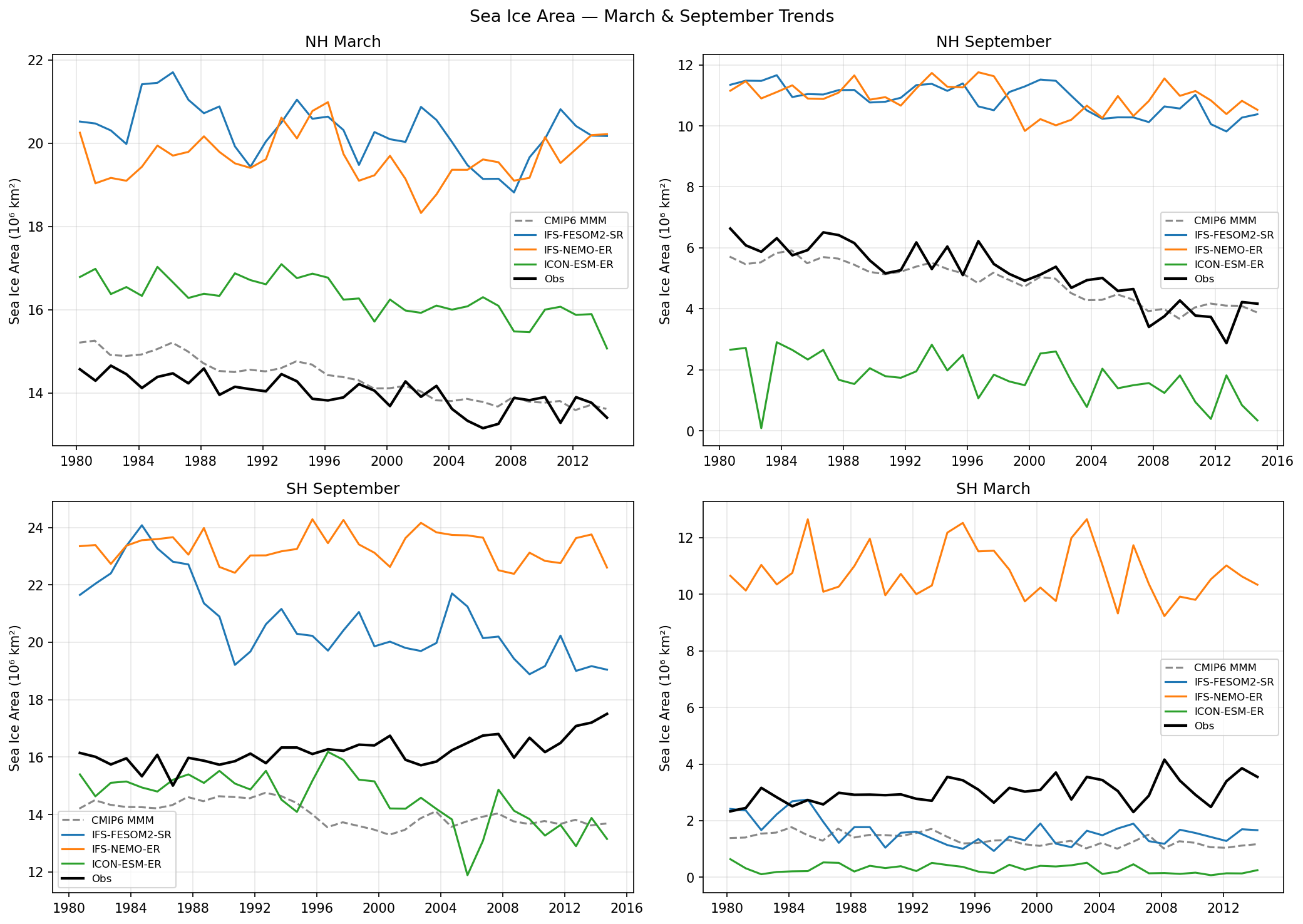
Sea Ice Area March & September Trends
| Variables | siconc, sithick |
|---|---|
| Models | IFS-FESOM2-SR, IFS-NEMO-ER, ICON-ESM-ER |
| Reference Dataset | OSI_SAF |
| Units | 0-1 |
| Period | 1980–2014 |
Summary high
This figure evaluates annual maximum and minimum sea ice area trends for the Northern and Southern Hemispheres, revealing severe biases in the high-resolution EERIE models compared to observations (OSI-SAF) and the CMIP6 multi-model mean. The IFS variants generally suffer from massive positive biases (too much ice), while ICON-ESM-ER exhibits exaggerated seasonality in the Arctic and general underestimation in the Antarctic.
Key Findings
- IFS-NEMO-ER and IFS-FESOM2-SR grossly overestimate NH sea ice area in both March and September by ~5-6 million km², placing their summer minimums (~11 million km²) well above the observed winter maximums in some years.
- IFS-NEMO-ER shows a catastrophic positive bias in the Antarctic summer (SH March), retaining over 10 million km² of ice compared to observations of ~3 million km², indicating a failure of seasonal melt.
- ICON-ESM-ER displays an amplified seasonal cycle in the NH: it overestimates the March maximum by ~2 million km² but severely underestimates the September minimum, approaching ice-free conditions (<2 million km²) well below observations.
- The CMIP6 Multi-Model Mean (MMM) tracks observations significantly better than the specific high-resolution simulations shown, particularly capturing the absolute magnitude and downward trend of NH September sea ice.
Spatial Patterns
The IFS biases manifest as large systematic offsets (roughly +6 million km² in NH) rather than trend errors. In the SH, IFS-FESOM2-SR exhibits a notable 'drift' or regime shift around 1988 in September, dropping from ~23 to ~19 million km², suggesting initialization shock. ICON-ESM-ER is consistently low in the SH.
Model Agreement
There is very poor agreement among models and with observations. The spread between models is extreme, exceeding 8 million km² in SH March—larger than the observational mean itself. The high-resolution models do not converge toward the CMIP6 baseline.
Physical Interpretation
The pervasive positive bias in IFS models suggests a strong cold bias in the atmosphere/ocean or incorrect sea ice albedo parameterizations preventing summer melt. The ICON pattern (excessive winter area, deficient summer area) implies the formation of extensive but thermodynamically thin ice that melts too easily. The IFS-FESOM drift implies the ocean state was still adjusting (spin-up) during the first decade of the run.
Caveats
- The extreme magnitude of biases (especially IFS-NEMO-ER in SH) suggests these specific model tunings are physically unrealistic for polar cryosphere studies.
- Drift in IFS-FESOM2-SR indicates the simulation may not be in equilibrium.
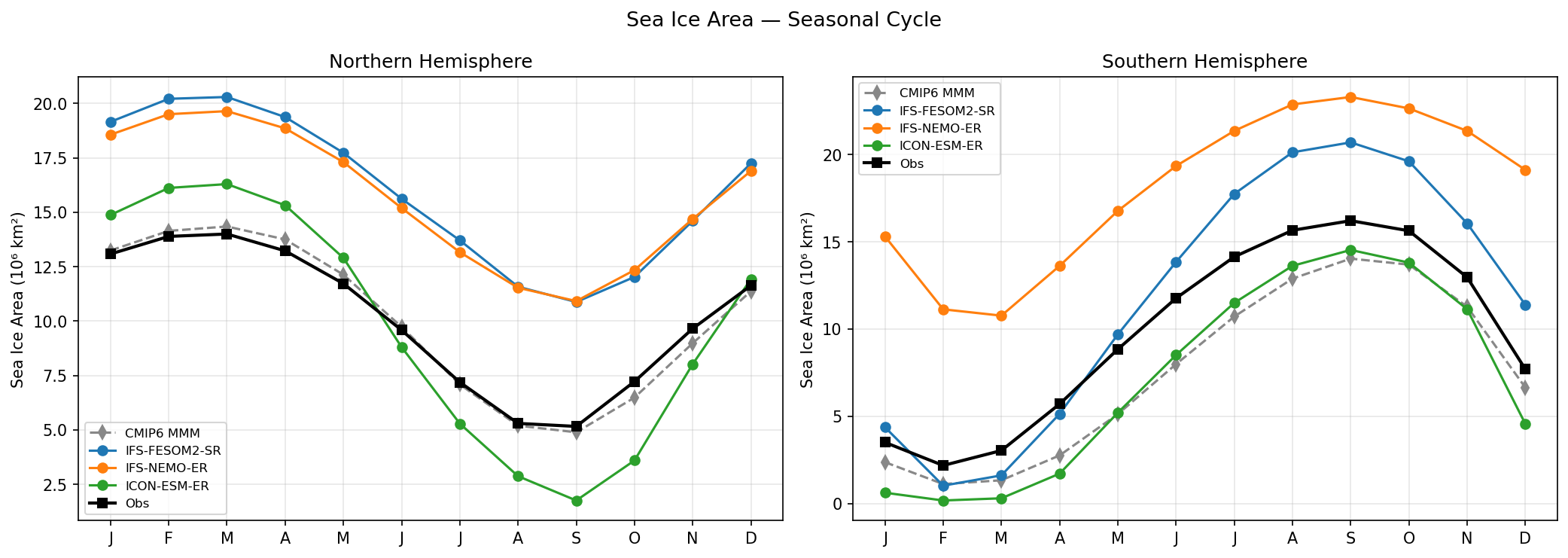
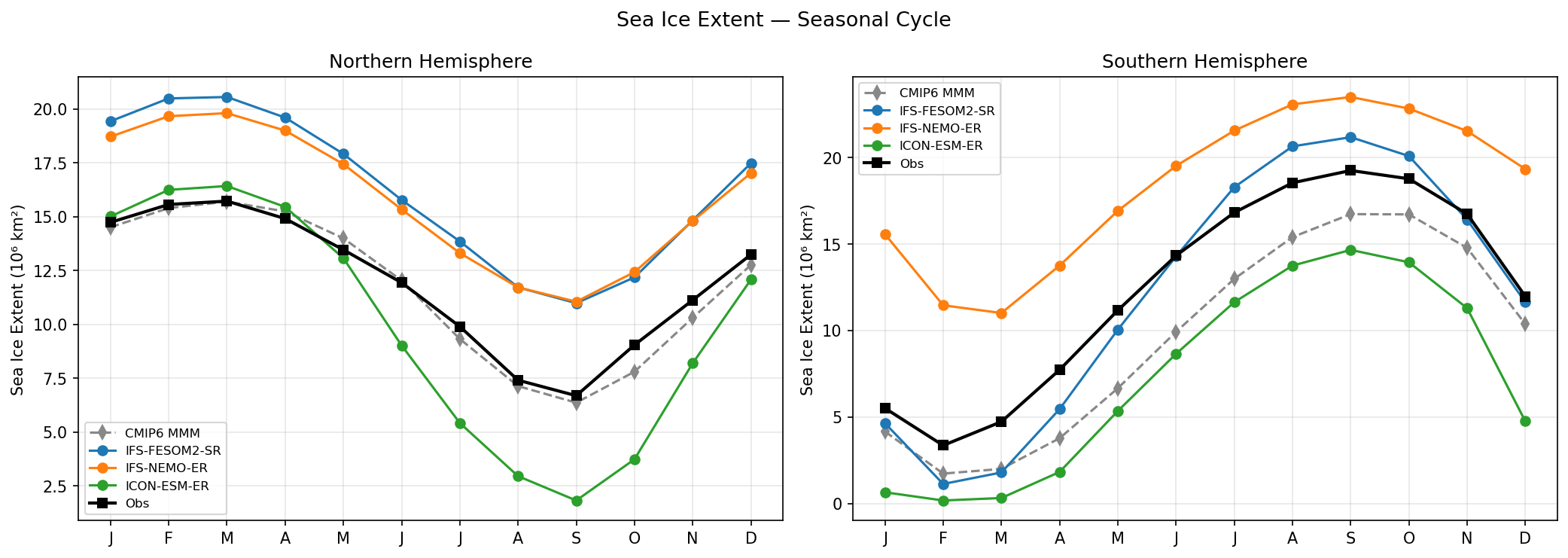
Sea Ice Area Seasonal Cycle
| Variables | siconc, sithick |
|---|---|
| Models | IFS-FESOM2-SR, IFS-NEMO-ER, ICON-ESM-ER |
| Reference Dataset | OSI_SAF |
| Units | 0-1 |
| Period | 1980–2014 |
Summary high
This diagnostic compares the seasonal cycle of Northern and Southern Hemisphere sea ice area from three high-resolution EERIE models against OSI-SAF observations and the CMIP6 multi-model mean. The models exhibit drastic biases: IFS configurations show massive overestimations of sea ice area, while ICON-ESM-ER tends to exaggerate seasonal amplitude in the North and underestimate area in the South.
Key Findings
- IFS-NEMO-ER and IFS-FESOM2-SR exhibit a severe, systematic positive bias in the Northern Hemisphere (NH), overestimating sea ice area by ~6 million km² year-round; their summer minimum (~11 million km²) is more than double the observed value (~5 million km²).
- In the Southern Hemisphere (SH), IFS-NEMO-ER maintains a huge positive bias throughout the year (+5 to +9 million km²). IFS-FESOM2-SR shows a similar winter overshoot but agrees well with observations during the summer minimum.
- ICON-ESM-ER displays an exaggerated seasonal cycle in the NH, with too much winter ice (~16 vs 14 million km²) and a severe underestimation of summer ice (<2 vs 5 million km²).
- The CMIP6 MMM significantly outperforms the high-resolution IFS models in the NH, tracking observations closely, but underestimates SH winter maxima, a bias shared by ICON-ESM-ER.
Spatial Patterns
While the phasing (timing of minima/maxima) is generally captured correctly—March/September for NH and February/September for SH—the amplitudes differ. IFS models in the NH show correct amplitude (~9 million km²) but a massive mean-state offset. ICON-ESM-ER in the NH shows an excessive amplitude (~14 million km²).
Model Agreement
Inter-model agreement is poor. The two IFS models (differing in ocean discretization) generally cluster with high positive biases, though they diverge in the SH summer. ICON-ESM-ER behaves distinctly, resembling the CMIP6 MMM pattern in the SH (low bias) but deviating in the NH (strong seasonal cycle).
Physical Interpretation
The systematic positive offset in IFS models suggests a profound cold bias in the polar regions or issues with initial conditions/drift retaining too much ice; the lack of summer melt reduction implies albedo or cloud feedback issues. ICON-ESM-ER's deep NH summer melt suggests a too-strong ice-albedo feedback or initially thin ice. The low SH bias in ICON/CMIP6 is consistent with the common 'warm Southern Ocean' bias, whereas IFS appears to have a 'cold Southern Ocean' or excessive freezing bias.
Caveats
- Figure evaluates area only, not volume/thickness; models with excessive area might still have realistic or too-low volume if ice is very thin.
- Large biases suggest these runs might be in drift or have significant tuning imbalances in polar energy budgets.
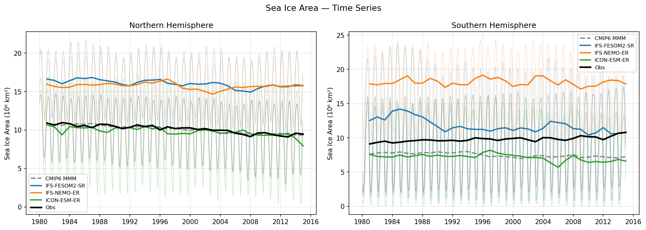
Sea Ice Area Time Series
| Variables | siconc, sithick |
|---|---|
| Models | IFS-FESOM2-SR, IFS-NEMO-ER, ICON-ESM-ER |
| Reference Dataset | OSI_SAF |
| Units | 0-1 |
| Period | 1980–2014 |
Summary high
Time series of Northern and Southern Hemisphere sea ice area (1980–2014) comparing three high-resolution models against OSI-SAF observations and the CMIP6 multi-model mean.
Key Findings
- ICON-ESM-ER shows excellent agreement with Northern Hemisphere (NH) observations, closely tracking the magnitude and negative trend of the CMIP6 MMM and OSI-SAF data.
- Both IFS-based models (IFS-FESOM2-SR and IFS-NEMO-ER) exhibit a massive positive bias in the NH, overestimating annual mean sea ice area by ~5-6 million km² (approx. 50% higher than observations).
- Southern Hemisphere (SH) results show large inter-model divergence: IFS-NEMO-ER drastically overestimates area (~18 vs 10 million km²), IFS-FESOM2-SR overestimates to a lesser degree, while ICON-ESM-ER underestimates area (~7 vs 10 million km²).
- IFS-FESOM2-SR displays a noticeable negative drift in the SH, decreasing from ~13 to ~11 million km² over the simulation period, suggesting equilibration issues.
Spatial Patterns
The Northern Hemisphere is characterized by a stable observational baseline with a slight decline, captured well by ICON but offset by a large constant bias in IFS models. The Southern Hemisphere shows high variability and stronger model disagreement, with IFS-NEMO-ER nearly doubling the observed ice area.
Model Agreement
Low inter-model agreement. The models cluster into two behaviors: ICON mimics the CMIP6 MMM (good NH, low SH), while the IFS family consistently predicts significantly more sea ice than observed in both hemispheres.
Physical Interpretation
The excessive sea ice in the IFS models suggests a systematic cold bias in high-latitude sea surface temperatures or aggressive sea ice formation/retention parameterizations. The underestimation of SH ice by ICON is a common feature in climate models (often linked to Warm Southern Ocean biases). The drift in IFS-FESOM2-SR SH ice implies the model is adjusting from its initial ocean state.
Caveats
- Sea ice area integrates concentration and extent but does not reveal thickness or volume errors.
- The analysis does not distinguish between summer minimum and winter maximum biases specifically, though the annual mean offset is dominant.
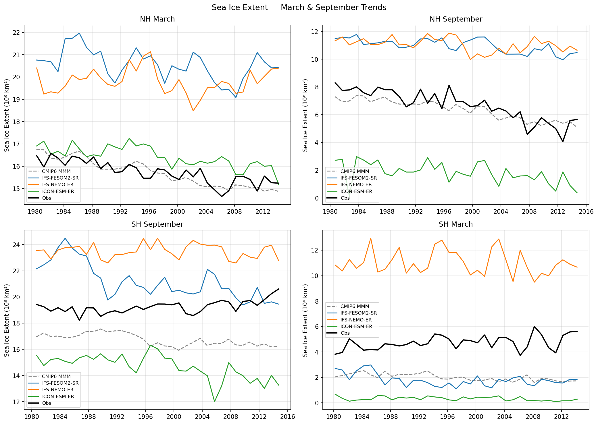
Sea Ice Extent March & September Trends
| Variables | siconc, sithick |
|---|---|
| Models | IFS-FESOM2-SR, IFS-NEMO-ER, ICON-ESM-ER |
| Reference Dataset | OSI_SAF |
| Units | 0-1 |
| Period | 1980–2014 |
Summary high
This figure evaluates annual sea ice extent trends for March and September in both hemispheres, revealing substantial biases in the high-resolution models compared to observations and the CMIP6 multi-model mean (MMM).
Key Findings
- IFS-NEMO-ER exhibits a massive systematic positive bias in sea ice extent across all seasons and hemispheres, most notably in SH March where extent is ~11 million km² vs. ~4 million km² in observations.
- IFS-FESOM2-SR shares the severe positive bias in the Northern Hemisphere (exceeding observations by ~5 million km² in both March and September) but switches to a negative bias in SH March (summer).
- ICON-ESM-ER performs best for NH March (winter max) extent, closely tracking observations, but suffers from severe negative biases in NH September (summer min) and throughout the Southern Hemisphere.
- None of the high-resolution models capture the strong observed decline in NH September sea ice as effectively as the CMIP6 MMM; the IFS models show flat trends with excessive ice, while ICON is essentially ice-free too early.
Spatial Patterns
The Northern Hemisphere is characterized by a stark bifurcation: the IFS models (NEMO and FESOM) simulate excessive ice cover year-round (~20M km² vs 16M km² in March), while ICON simulates excessive summer melting. In the Southern Hemisphere, inter-model divergence is extreme during the summer minimum (March), with IFS-NEMO-ER retaining unrealistic ice cover while ICON and IFS-FESOM2-SR deplete it below observational levels.
Model Agreement
There is very poor inter-model agreement. The models bracket the observations with large errors in opposite directions (IFS models too high, ICON too low), whereas the lower-resolution CMIP6 MMM often provides a better fit to the observed magnitude and trends, particularly in the NH.
Physical Interpretation
The positive biases in the IFS models (particularly NEMO) suggest a cold bias in polar SSTs or sea ice thermodynamics (e.g., albedo parameters) that prevents adequate summer melting. Conversely, ICON-ESM-ER likely has a 'warm' bias or excessive surface melt efficiency, leading to an amplified seasonal cycle in the NH and general ice deficiency in the SH. The lack of NH September trend in IFS models implies they are insufficiently sensitive to radiative forcing or buffered by excessive ice thickness.
Caveats
- The figure shows extent only; volume/thickness data would determine if the 'excessive' ice in IFS models is thin and widely spread or physically thick.
- The massive biases in the IFS models suggest they may be in a spin-up drift phase or suffer from initialization shocks compared to the equilibrium assumptions of the observations.
Sea Ice Extent Seasonal Cycle
| Variables | siconc, sithick |
|---|---|
| Models | IFS-FESOM2-SR, IFS-NEMO-ER, ICON-ESM-ER |
| Reference Dataset | OSI_SAF |
| Units | 0-1 |
| Period | 1980–2014 |
Summary high
This figure evaluates the seasonal cycle of Northern and Southern Hemisphere sea ice extent for three high-resolution coupled models against OSI-SAF observations and the CMIP6 multi-model mean. The models exhibit large, divergent biases, with IFS variants generally overestimating extent and ICON-ESM-ER tending towards excessive melting, particularly in summer.
Key Findings
- IFS-FESOM2-SR and IFS-NEMO-ER show a systematic positive bias in the Northern Hemisphere, overestimating extent by ~4–5 × 10⁶ km² year-round compared to observations.
- ICON-ESM-ER captures the NH winter maximum well (~16 × 10⁶ km²) but suffers from extreme summer melt, dropping to <2 × 10⁶ km² in September (vs ~6.5 × 10⁶ km² in observations), implying a nearly ice-free summer Arctic.
- In the Southern Hemisphere, inter-model spread is extreme: IFS-NEMO-ER vastly overestimates ice (winter max >23 × 10⁶ km²), while ICON-ESM-ER severely underestimates it year-round (winter max <15 × 10⁶ km²).
Spatial Patterns
The seasonal phase is generally correct across models (maxima in March/September), but mean states differ fundamentally. The NH biases for IFS models are relatively constant offsets, whereas ICON shows a strong amplitude bias (correct winter, too low summer). In the SH, IFS-NEMO-ER fails to melt back sufficiently in summer (Feb), retaining ~11 × 10⁶ km² vs ~3.5 × 10⁶ km² observed.
Model Agreement
Inter-model agreement is very low, with spreads exceeding 50% of the mean value in some seasons. The CMIP6 MMM baseline often outperforms the individual high-resolution simulations, particularly in the NH where it tracks observations closely.
Physical Interpretation
The shared positive bias in NH for both IFS-based models suggests a common atmospheric driver (e.g., cold bias) or sea ice tuning that favors excessive growth/retention. Conversely, ICON-ESM-ER appears to have overly strong positive feedbacks (likely ice-albedo) or insufficient ocean stratification/too warm ocean temperatures, leading to rapid summer loss in the NH and inhibited growth in the SH.
Caveats
- Sea ice extent (area with >15% concentration) does not reflect ice thickness or volume, which might show different bias patterns.
- Observational uncertainty exists in melt ponds/summer retrieval, but model biases here (up to 5-10 million km²) far exceed instrument error.
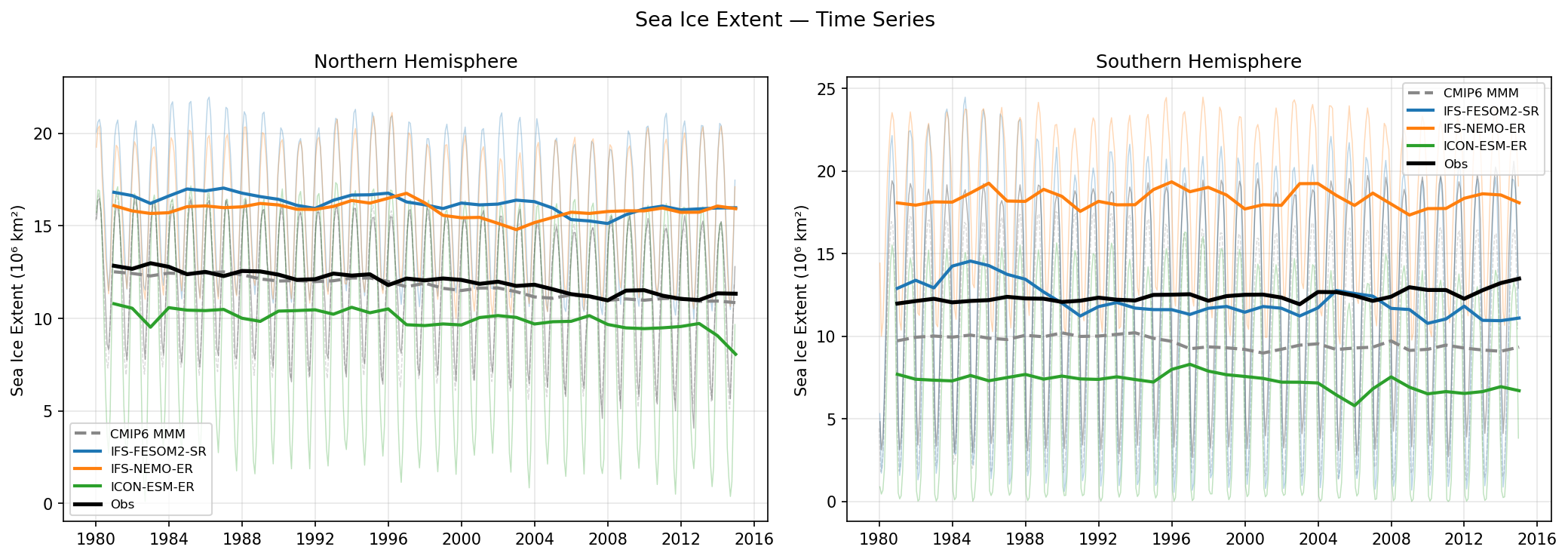
Sea Ice Extent Time Series
| Variables | siconc, sithick |
|---|---|
| Models | IFS-FESOM2-SR, IFS-NEMO-ER, ICON-ESM-ER |
| Reference Dataset | OSI_SAF |
| Units | 0-1 |
| Period | 1980–2014 |
Summary high
Time series of Northern (NH) and Southern Hemisphere (SH) sea ice extent (1980–2015) comparing three high-resolution models against OSI-SAF observations and the CMIP6 multi-model mean (MMM).
Key Findings
- In the NH, both IFS-based models (IFS-FESOM2-SR, IFS-NEMO-ER) exhibit a substantial positive bias (annual mean ~16 vs 12 million km²), primarily driven by excessive winter maxima (>20 million km²).
- ICON-ESM-ER displays a consistent negative bias in both hemispheres, underestimating annual mean extent by ~2 million km² in the NH and ~5 million km² in the SH.
- In the SH, model spread is extreme: IFS-NEMO-ER overestimates extent by ~50%, ICON-ESM-ER underestimates by ~40%, while IFS-FESOM2-SR shows remarkable agreement with observations, outperforming the negatively biased CMIP6 MMM.
- The observed NH decline trend is captured well by the CMIP6 MMM and ICON-ESM-ER, whereas the IFS variants show weaker downward trends.
Spatial Patterns
Seasonal cycles (thin lines) reveal that the NH positive bias in IFS models is dominated by extensive winter sea ice growth (reaching >20 million km²), suggesting ice extending into normally ice-free sub-polar regions. In the SH, IFS-NEMO-ER maintains a high bias year-round, while ICON-ESM-ER's minima are extremely low, approaching near-ice-free summer conditions in some years.
Model Agreement
Inter-model agreement is very poor, particularly in the Southern Hemisphere where the spread between the highest (IFS-NEMO-ER) and lowest (ICON-ESM-ER) models exceeds 10 million km². IFS-FESOM2-SR is the only model that closely matches SH observations.
Physical Interpretation
The divergence between IFS-FESOM2-SR and IFS-NEMO-ER in the SH suggests that ocean model formulation (FESOM vs. NEMO) critically controls Antarctic sea ice simulation, as both share the same atmospheric component. The high bias in IFS-NEMO-ER implies a too-cold Southern Ocean surface or excessive stratification preventing deep heat convection. Conversely, ICON's ubiquitous low bias points to a global warm bias in polar regions or insufficient sea ice formation/retention physics.
Caveats
- Extent is an integrated metric and does not reveal regional compensation errors (e.g., too much ice in one sector, too little in another).
- Does not assess sea ice thickness or volume, which often show different bias patterns.
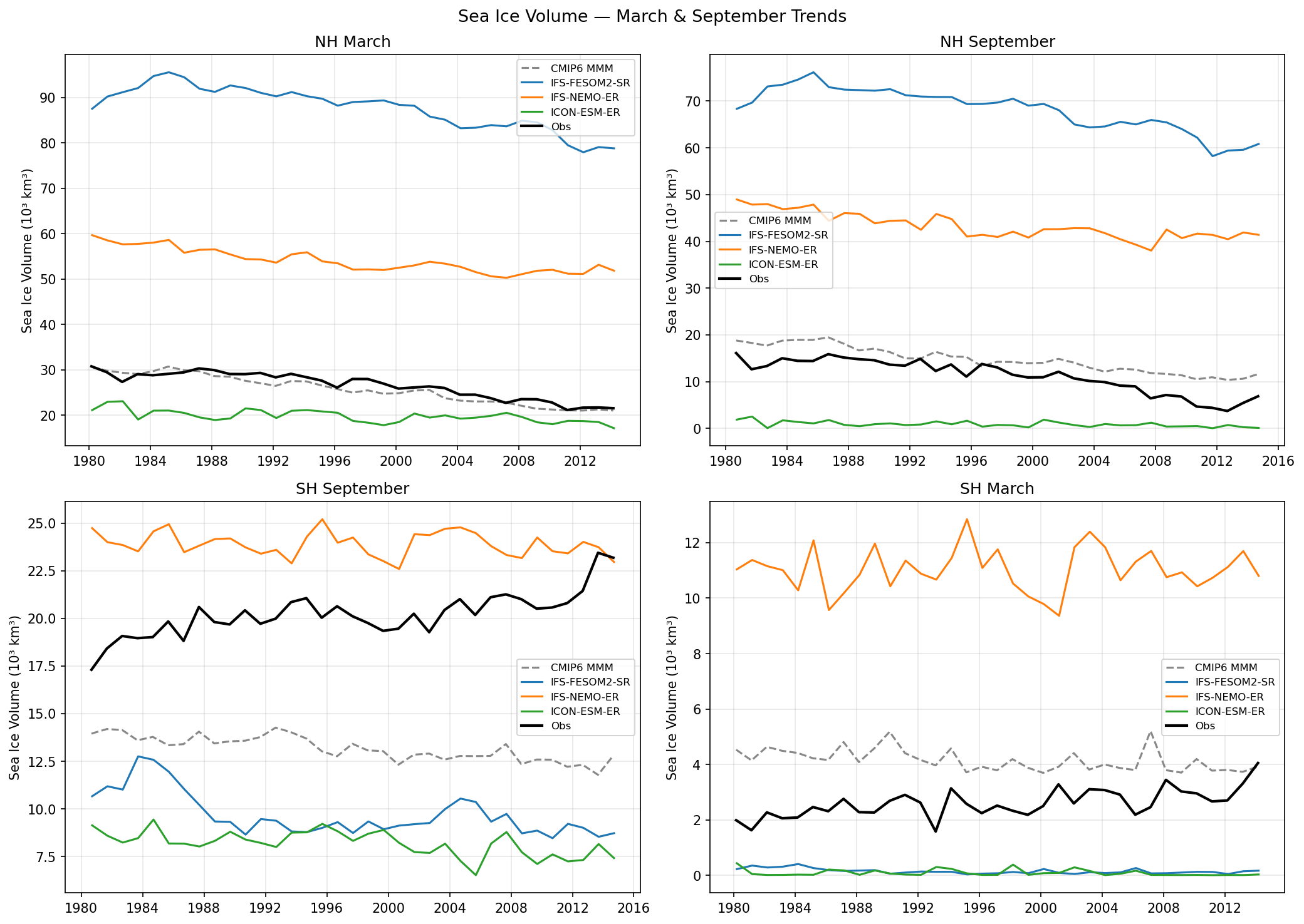
Sea Ice Volume March & September Trends
| Variables | siconc, sithick |
|---|---|
| Models | IFS-FESOM2-SR, IFS-NEMO-ER, ICON-ESM-ER |
| Reference Dataset | PSC |
| Units | 0-1 |
| Period | 1980–2014 |
Summary high
Time series analysis of Northern and Southern Hemisphere sea ice volume trends for March and September (1980–2014). The models exhibit extreme inter-model spread and significant biases compared to observations (likely PIOMAS/GIOMAS reanalysis) and the CMIP6 multi-model mean.
Key Findings
- IFS-FESOM2-SR and IFS-NEMO-ER show massive positive biases in Northern Hemisphere (NH) sea ice volume; IFS-FESOM2-SR exceeds observations by a factor of 3–4, indicating excessive multi-year ice accumulation.
- ICON-ESM-ER consistently underestimates sea ice volume globally, resulting in a nearly ice-free Arctic in September (< 2 × 10³ km³) throughout the simulation period.
- In the Southern Hemisphere (SH), biases diverge: IFS-NEMO-ER overestimates volume (particularly the summer minimum), while IFS-FESOM2-SR and ICON-ESM-ER significantly underestimate the winter maximum compared to observations.
- While CMIP6 MMM tracks observational magnitudes reasonably well (though biased low in SH winter), the high-resolution models evaluated here deviate more significantly from the observational reference.
Spatial Patterns
The NH shows a declining trend in all datasets, consistent with Arctic warming, though the absolute baselines in IFS models are shifted drastically upwards. In the SH, observations show a slight positive trend (pre-2015), which is not clearly captured by the models; IFS-NEMO-ER maintains a high, stable volume, while others remain low.
Model Agreement
Very poor agreement between models and observations, and among models themselves. The spread in NH September volume (~0 to ~70 × 10³ km³) dwarfs the observational mean (~5–15 × 10³ km³).
Physical Interpretation
The extreme NH volume in IFS-FESOM2-SR suggests a thermodynamic imbalance leading to unrealistic thickening of multi-year ice, possibly due to albedo tuning or insufficient ocean-to-ice heat flux. Conversely, ICON-ESM-ER's low bias suggests excessive surface melting or strong ocean heat transport. In the SH, IFS-NEMO-ER's retention of summer ice (high March volume) implies issues with austral summer melt processes or mixed-layer physics, whereas the other models likely suffer from Southern Ocean warm biases preventing ice expansion.
Caveats
- Sea ice volume is not directly observed globally; 'Obs' likely refers to a reanalysis product like PIOMAS (NH) and GIOMAS (SH), which carries its own model-dependent uncertainties.
- The vertical axis scales differ significantly between NH and SH panels, masking the fact that SH volume errors are smaller in absolute terms than the massive NH outliers.
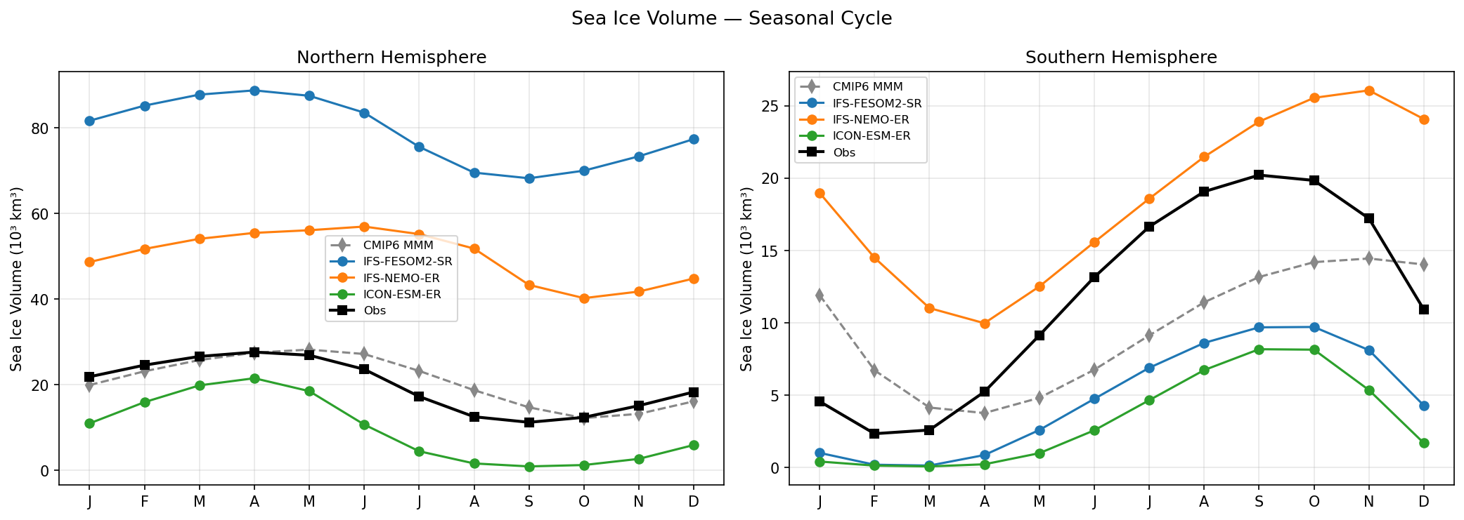
Sea Ice Volume Seasonal Cycle
| Variables | siconc, sithick |
|---|---|
| Models | IFS-FESOM2-SR, IFS-NEMO-ER, ICON-ESM-ER |
| Reference Dataset | PSC |
| Units | 0-1 |
| Period | 1980–2014 |
Summary high
This figure displays the seasonal cycle of Northern (NH) and Southern Hemisphere (SH) sea ice volume ($10^3$ km$^3$). It reveals massive inter-model discrepancies, with IFS-based models showing significant volume overestimations in the NH, while ICON-ESM-ER generally underestimates volume, particularly in the NH summer.
Key Findings
- IFS-FESOM2-SR exhibits an extreme positive bias in NH sea ice volume, ranging from 70–90 $10^3$ km$^3$, roughly 3–4 times the observational reference (~20–30 $10^3$ km$^3$).
- IFS-NEMO-ER also significantly overestimates NH volume (approx. double observations) and is the only model to overestimate SH volume, particularly during the austral summer minimum.
- ICON-ESM-ER generally underestimates sea ice volume; in the NH, it tracks observations in winter but melts nearly completely in summer (near-zero volume), while in the SH, it produces less than half the observed peak volume.
- The CMIP6 Multi-Model Mean (MMM) agrees reasonably well with observations in the NH, outperforming the high-resolution EERIE models, but underestimates peak volume in the SH.
Spatial Patterns
In the NH, the seasonal phase is generally captured by all models (max in Apr, min in Sept), but the mean state offsets are enormous. In the SH, IFS-NEMO-ER shows a distorted seasonal cycle with a very high summer minimum (~10 $10^3$ km$^3$ vs ~2.5 $10^3$ km$^3$ observed), suggesting excessive retention of multi-year ice.
Model Agreement
Inter-model agreement is very poor, with volume estimates differing by factors of 3-4. The high-resolution models generally deviate more from observations than the CMIP6 MMM ensemble average.
Physical Interpretation
The massive NH volume overestimates in IFS-FESOM2-SR and IFS-NEMO-ER imply excessive ice thickness, likely due to imbalances in thermodynamic growth/melt rates or albedo tuning, rather than just area biases. Conversely, ICON-ESM-ER's 'thin ice' bias (near-zero NH summer volume) suggests excessive surface melting or insufficient winter growth. The SH behavior of IFS-NEMO-ER suggests a failure to melt first-year ice during summer, leading to artificial multi-year ice accumulation.
Caveats
- Sea ice volume observations are typically derived from reanalyses (e.g., PIOMAS/GIOMAS) rather than direct satellite measurement, carrying higher uncertainty than concentration/extent data.
- The prompt metadata lists 'siconc' as the variable, but the plot clearly shows volume, implying thickness is integrated.
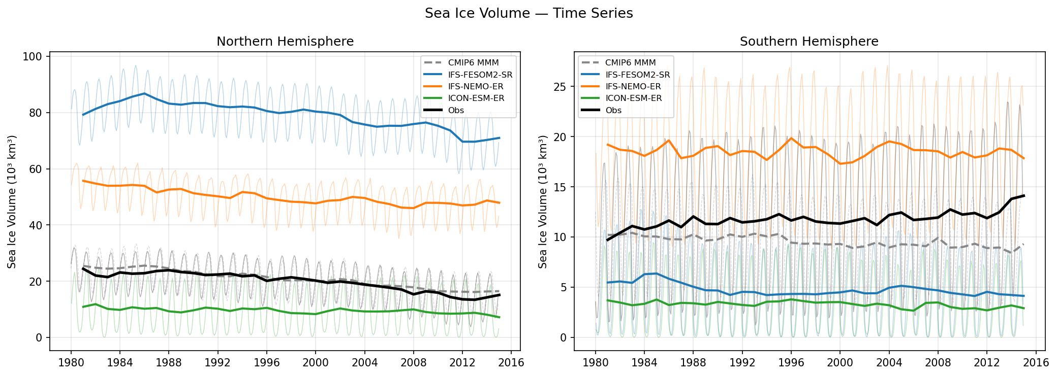
Sea Ice Volume Time Series
| Variables | siconc, sithick |
|---|---|
| Models | IFS-FESOM2-SR, IFS-NEMO-ER, ICON-ESM-ER |
| Reference Dataset | PSC |
| Units | 0-1 |
| Period | 1980–2014 |
Summary high
The figure displays time series of Northern (NH) and Southern Hemisphere (SH) sea ice volume from 1980–2015, revealing substantial biases in the high-resolution EERIE models compared to observations and the CMIP6 Multi-Model Mean (MMM). While the CMIP6 MMM tracks observational magnitudes relatively well, the evaluated models exhibit massive spread, with IFS-FESOM2-SR and IFS-NEMO-ER generally overestimating volume (particularly in the NH) and ICON-ESM-ER consistently underestimating it.
Key Findings
- In the NH, IFS-FESOM2-SR shows an extreme positive bias, simulating volumes (~80 × 10³ km³) nearly 4 times larger than observations (~20–25 × 10³ km³).
- IFS-NEMO-ER also significantly overestimates NH volume (~50–55 × 10³ km³), roughly double the observational estimate.
- ICON-ESM-ER consistently underestimates sea ice volume in both hemispheres, with NH values (~10 × 10³ km³) approximately 50% of observations.
- In the SH, IFS-NEMO-ER overestimates volume (~18 × 10³ km³ vs ~10–12 × 10³ km³ obs), while IFS-FESOM2-SR and ICON-ESM-ER significantly underestimate it (~3–5 × 10³ km³).
- The CMIP6 MMM aligns much closer to the observational reference (black line) in magnitude for both hemispheres than any of the specific high-resolution simulations shown.
Spatial Patterns
The Northern Hemisphere shows a clear downward trend in the observations and CMIP6 MMM, which is weakly replicated in the biased model baselines (though IFS-FESOM2-SR's trend is somewhat flatter). The Southern Hemisphere observations show a slight increase in volume over the period, which is not clearly captured by the models; IFS-NEMO-ER shows a slight decline, while others are relatively flat.
Model Agreement
Inter-model agreement is very poor, with an order-of-magnitude difference in NH volume between IFS-FESOM2-SR and ICON-ESM-ER. The models diverge significantly from the CMIP6 MMM baseline, suggesting that increased resolution in these specific configurations has not converged to a more accurate mean state for sea ice volume.
Physical Interpretation
Since sea ice extent is generally better constrained by satellite data, the massive volume discrepancies point primarily to sea ice thickness biases. The extreme volume in IFS-FESOM2-SR (NH) suggests excessive thermodynamic growth or dynamic ridging/retention of thick ice (possibly due to grid-specific rheology or insufficient export). Conversely, ICON-ESM-ER likely suffers from excessive melt or insufficient thickness accretion. The contrast between IFS-FESOM2 and IFS-NEMO (sharing an atmospheric component) highlights that the ocean/sea-ice component formulation (FESOM2 vs. NEMO/SI3) is the dominant driver of these differences.
Caveats
- Observations for sea ice volume are typically derived from reanalyses (e.g., PIOMAS for NH) rather than direct observation; the metadata 'PSC (ice_conc)' likely refers only to the concentration input, as volume requires thickness estimates.
- The massive biases (400% in some cases) obscure the analysis of inter-annual variability and trend sensitivity.
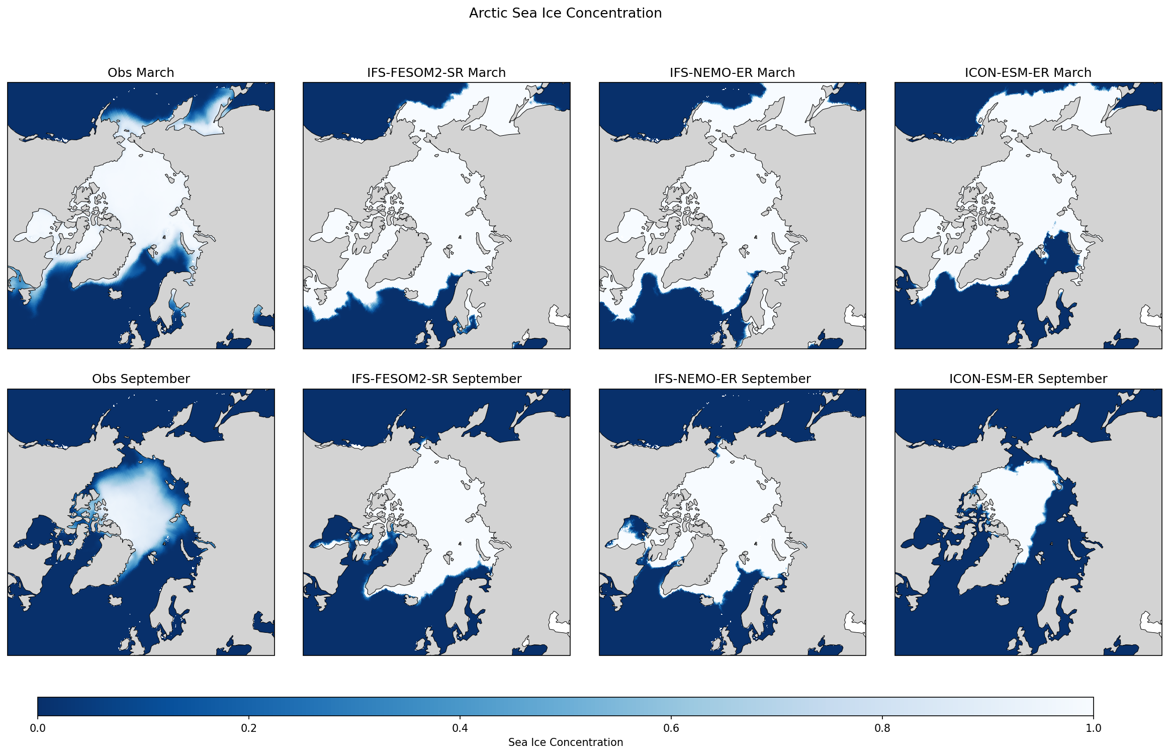
Arctic Sea Ice Concentration
| Variables | siconc |
|---|---|
| Models | IFS-FESOM2-SR, IFS-NEMO-ER, ICON-ESM-ER |
| Reference Dataset | OSI_SAF |
| Units | 0-1 |
| Period | 1980–2014 |
Summary high
This diagnostic compares Arctic sea ice concentration climatologies (March and September) from three high-resolution coupled models against OSI-SAF observations. IFS-FESOM2-SR demonstrates the best overall agreement with observations, while IFS-NEMO-ER and ICON-ESM-ER exhibit significant negative biases in specific seasons and regions.
Key Findings
- IFS-FESOM2-SR captures the spatial distribution of sea ice most accurately, reproducing both the winter extension into the Labrador Sea and the summer minimum extent well.
- IFS-NEMO-ER consistently underestimates sea ice concentration, with a retreated winter ice edge in the Barents/Labrador Seas and a severe underestimation of the September minimum, where the pack is significantly reduced and fragmented compared to observations.
- ICON-ESM-ER shows a strong 'warm winter' bias in the Atlantic sector, failing to form ice in the Labrador Sea and much of the Barents Sea in March, yet paradoxically maintains a robust, highly concentrated central ice pack in September.
Spatial Patterns
In March (winter maximum), the primary discrepancies are in the Atlantic marginal ice zones: observations show ice extending south to Newfoundland (Labrador Sea) and covering the Barents Sea. IFS-NEMO-ER and ICON-ESM-ER retreat the ice edge significantly northward in these regions. In September (summer minimum), models tend to show sharper gradients (binary 100% vs 0% concentration) compared to the diffuse marginal ice zone seen in observations. IFS-NEMO-ER exhibits a distinct 'hole' or severe thinning in the Eurasian sector of the Arctic basin in summer.
Model Agreement
Inter-model agreement is low, particularly in the marginal seas. IFS-FESOM2-SR aligns closely with observations, whereas IFS-NEMO-ER and ICON-ESM-ER diverge significantly from observations and each other, representing different failure modes (year-round underestimation vs. seasonal/regional contrast).
Physical Interpretation
The lack of winter ice in the Labrador and Barents Seas in IFS-NEMO-ER and ICON-ESM-ER suggests excessive oceanic heat transport from the North Atlantic (Atlantification) or warm atmospheric biases preventing ice formation. The severe summer melt in IFS-NEMO-ER indicates strong positive feedback loops (ice-albedo) or insufficient vertical stratification allowing sub-surface heat to erode the pack. The sharp concentration gradients in models compared to observations likely reflect both model parameterization of sub-grid ice thickness and the difficulty of satellite retrievals in distinguishing melt ponds from open water.
Caveats
- Satellite observations in September may underestimate ice concentration due to melt ponds on the ice surface being interpreted as open water.
- The 0-1 scale masks differences in ice thickness; a model could have 100% concentration but very thin ice.
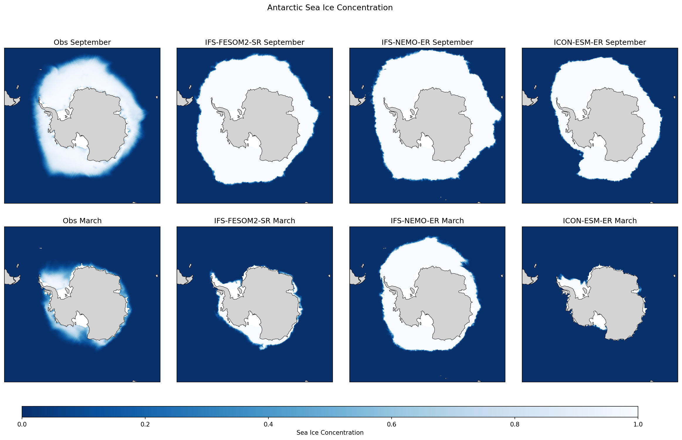
Antarctic Sea Ice Concentration
| Variables | siconc |
|---|---|
| Models | IFS-FESOM2-SR, IFS-NEMO-ER, ICON-ESM-ER |
| Reference Dataset | OSI_SAF |
| Units | 0-1 |
| Period | 1980–2014 |
Summary high
This figure compares spatial maps of Antarctic sea ice concentration for the austral winter maximum (September) and summer minimum (March) from three high-resolution models against OSI-SAF observations. It reveals extreme divergence in model performance, particularly regarding the amplitude of the seasonal cycle.
Key Findings
- IFS-NEMO-ER exhibits a severe positive bias in sea ice extent, most critically in March where it fails to melt back, retaining a near-winter extent that completely covers the Southern Ocean.
- IFS-FESOM2-SR and ICON-ESM-ER simulate the September maximum extent reasonably well compared to observations, though with sharper gradients at the ice edge.
- Conversely, IFS-FESOM2-SR and ICON-ESM-ER underestimate the March minimum, showing almost complete sea ice loss in the Weddell and Ross Seas where observations retain significant pack ice.
Spatial Patterns
Observations show a diffuse marginal ice zone with concentrations tapering off at the edge, whereas all models tend to simulate very high concentrations (near 100%) within the pack with sharper transitions to open water. In March, the observational 'survival' zones in the Weddell and Ross gyres are missed by FESOM and ICON (too little ice) and overwhelmed by NEMO (pan-Antarctic coverage).
Model Agreement
There is very poor inter-model agreement. The models split into two distinct failure modes: IFS-NEMO-ER has a 'permanently frozen' Southern Ocean with minimal seasonal cycle, while IFS-FESOM2-SR and ICON-ESM-ER have excessive seasonal cycles with realistic winter maxima but excessive summer melt.
Physical Interpretation
The massive persistent ice in IFS-NEMO-ER suggests a strong cold bias in the Southern Ocean surface layers, possibly due to insufficient vertical mixing of warm Circumpolar Deep Water or errors in surface energy balance (e.g., cloud radiative forcing). The excessive melt in FESOM and ICON implies strong positive ice-albedo feedbacks or warm atmospheric biases during the austral summer. The high concentration within the pack across all models suggests potential deficiencies in lead formation or rheology at this resolution.
Caveats
- The figure represents climatological means; interannual variability is not assessed.
- Satellite concentration retrievals have higher uncertainty during the melt season, though the model discrepancies here far exceed observational uncertainty.
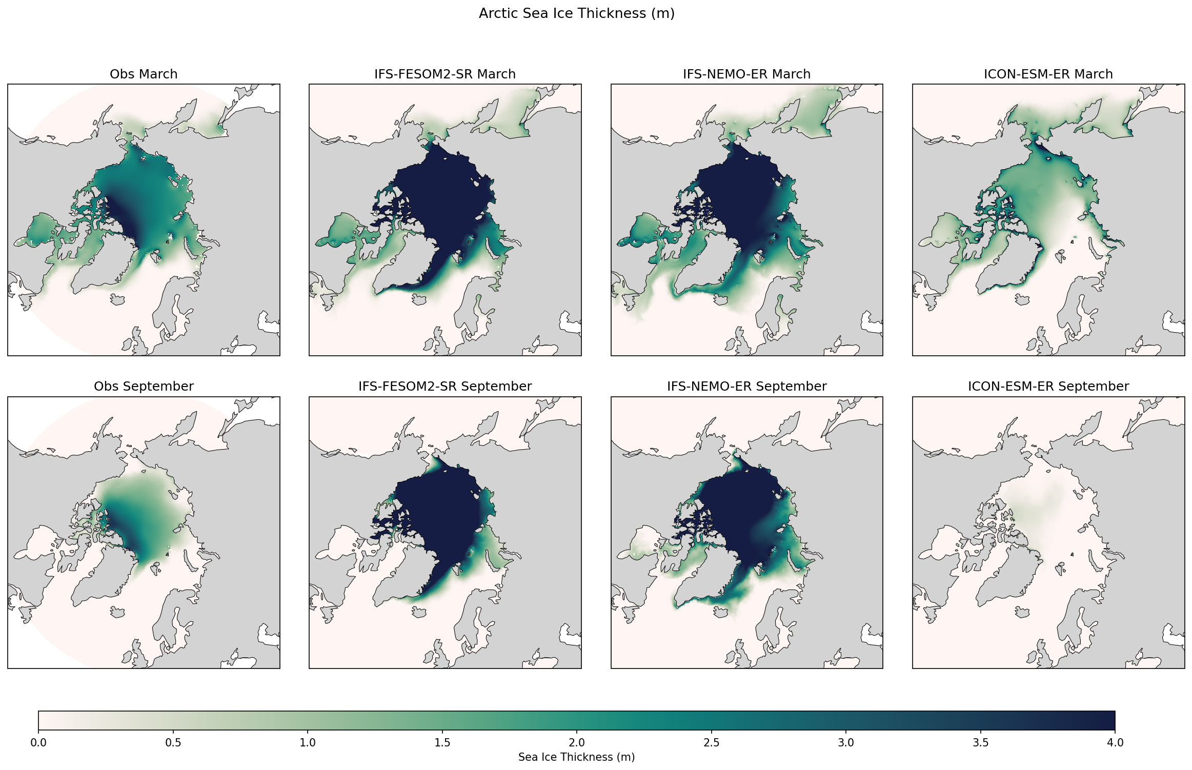
Arctic Sea Ice Thickness (m)
| Variables | sithick |
|---|---|
| Models | IFS-FESOM2-SR, IFS-NEMO-ER, ICON-ESM-ER |
| Reference Dataset | PSC |
| Units | m |
| Period | 1980–2014 |
Summary high
This figure evaluates Arctic sea ice thickness in March (annual maximum) and September (annual minimum) for three high-resolution models against observations (likely PIOMAS reanalysis). The models exhibit starkly contrasting biases: both IFS-based models significantly overestimate ice thickness, while ICON-ESM-ER significantly underestimates it.
Key Findings
- IFS-FESOM2-SR and IFS-NEMO-ER exhibit a strong positive thickness bias, simulating widespread central Arctic ice exceeding 3.5–4.0 m in March, whereas observations show such thickness is confined to the region north of the Canadian Archipelago.
- ICON-ESM-ER exhibits a severe negative thickness bias, with March thickness rarely exceeding 2.0 m in the central basin and a near-total loss of sea ice in September (almost ice-free conditions).
- Both IFS models retain excessive thick ice (>3.0 m) throughout the summer (September), showing limited seasonal sensitivity compared to the observed retreat.
- The spatial gradient of thickness (thickest near Canadian/Greenland coast, thinning towards Siberia) is poorly represented in all models; IFS models show a 'homogenized' thick central basin, while ICON is uniformly thin.
Spatial Patterns
Observations show a characteristic wedge of thick multi-year ice (>3 m) north of Greenland and the Canadian Archipelago, thinning towards the Siberian coast. IFS-FESOM2-SR and IFS-NEMO-ER extend this thick zone across the entire central Arctic basin, creating a massive area of ice >3.5 m. Conversely, ICON-ESM-ER fails to maintain this thick reservoir even in March, leading to a thin, fragile ice pack that largely vanishes in September.
Model Agreement
There is very low inter-model agreement. The models bifurcate into two extremes: the IFS-driven models (using FESOM and NEMO oceans) are 'too cold/thick', while the ICON model is 'too warm/thin'. None of the models closely reproduce the observational magnitude of sea ice thickness, though the IFS models capture the March spatial extent boundaries better than ICON captures the September extent.
Physical Interpretation
The excessive thickness in IFS-FESOM2 and IFS-NEMO suggests either insufficient summer melting (albedo feedback, cloud radiative forcing) or excessive thermodynamic growth/dynamic convergence. The similarity between the two IFS variants implies the atmospheric driver (IFS) or common tuning may dominate over ocean model differences (FESOM vs. NEMO). The thinning in ICON-ESM-ER suggests overly efficient ocean heat transport to the surface, insufficient insulation, or biases in surface energy balance leading to rapid melt. The lack of thick multi-year ice in ICON indicates the model fails to survive the melt season to build up thickness over years.
Caveats
- The 'Obs' dataset is not specified but is likely a reanalysis product like PIOMAS, as direct satellite thickness observations (e.g., CryoSat-2) are limited for the 1980–2014 period.
- Averaging over 1980–2014 masks the strong observed trend of thinning ice; however, the model biases are large enough to be distinct from trend-related errors.
Antarctic Sea Ice Thickness (m)
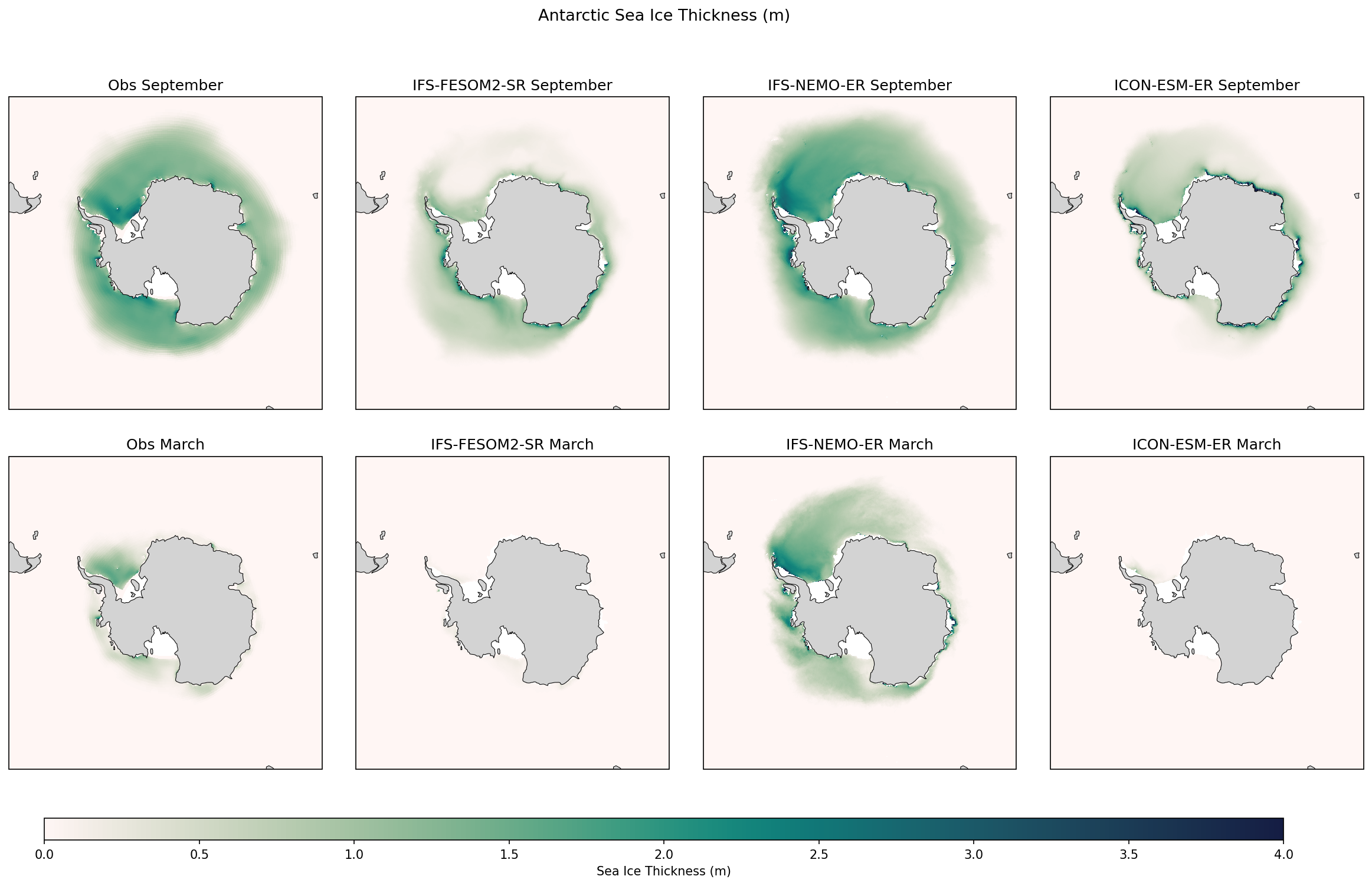
| Variables | sithick |
|---|---|
| Models | IFS-FESOM2-SR, IFS-NEMO-ER, ICON-ESM-ER |
| Reference Dataset | PSC |
| Units | m |
| Period | 1980–2014 |
Summary high
This figure evaluates Antarctic sea ice thickness climatologies for September (winter max) and March (summer min) across three high-resolution coupled models against observations. The models exhibit widely divergent behaviors, ranging from severe underestimation (ICON-ESM-ER) to potential overestimation of Weddell Sea thickness (IFS-NEMO-ER).
Key Findings
- ICON-ESM-ER shows a drastic negative bias in Antarctic sea ice, with winter (September) ice confined to a thin (<1m) coastal strip and almost zero ice surviving in summer (March).
- IFS-NEMO-ER simulates the most robust sea ice pack, producing thick ice (>2.5m) in the Weddell Sea that persists through the summer melt, appearing to overestimate thickness and extent compared to the observational reference.
- IFS-FESOM2-SR captures the spatial structure of winter sea ice better than ICON but generally underestimates thickness and fails to retain significant summer ice in the Weddell Sea compared to observations.
- Inter-model spread is extremely high, indicating significant structural or tuning differences in the sea ice components or Southern Ocean states of these coupled systems.
Spatial Patterns
In observations, thickest ice is found in the Weddell Sea (piled against the Antarctic Peninsula) and the Amundsen/Ross sectors. IFS-NEMO-ER reproduces and exaggerates this Weddell Sea accumulation, showing a massive wedge of multi-year ice. Conversely, ICON-ESM-ER lacks any significant ice away from the coast. IFS-FESOM2-SR shows a zonal band of ice but misses the thick accumulation zones.
Model Agreement
Model agreement is very low. The three models present three distinct regimes: excessive/thick (IFS-NEMO), intermediate/thin (IFS-FESOM), and deficient/sparse (ICON). None match the observational reference closely in both seasons.
Physical Interpretation
The accumulation of thick ice in the Weddell Sea in IFS-NEMO-ER suggests a strong representation of the Weddell Gyre circulation and convergent ice rheology, possibly combined with a cold bias or excessive ice growth. The near-total absence of pack ice in ICON-ESM-ER likely stems from a significant warm bias in Southern Ocean SSTs or issues with the ice formation parameterization. The difference between IFS-NEMO and IFS-FESOM (which share the same atmosphere) points to the ocean-ice component (NEMO-LIM/SI3 vs. FESOM) as the primary driver of these discrepancies.
Caveats
- Antarctic sea ice thickness observations (labeled 'Obs') generally have higher uncertainty than Arctic data; the concentric artifacts in the Obs panel suggest a reanalysis or interpolated product rather than direct altimetry.
- The 'Obs' reference appears to show more moderate thickness than IFS-NEMO but more extent than ICON, serving as a middle ground.