Evaluation Seasonal Cycle CMIP6
CMIP6 Multi-Model Mean Context
Comparison with CMIP6 ensemble mean from 11 members.
Contributing models: ACCESS-ESM1-5, AWI-CM-1-1-MR, CNRM-CM6-1, CNRM-ESM2-1, EC-Earth3, FGOALS-g3, GISS-E2-1-G, INM-CM5-0, IPSL-CM6A-LR, MPI-ESM1-2-LR, MRI-ESM2-0
Synthesis
Related diagnostics
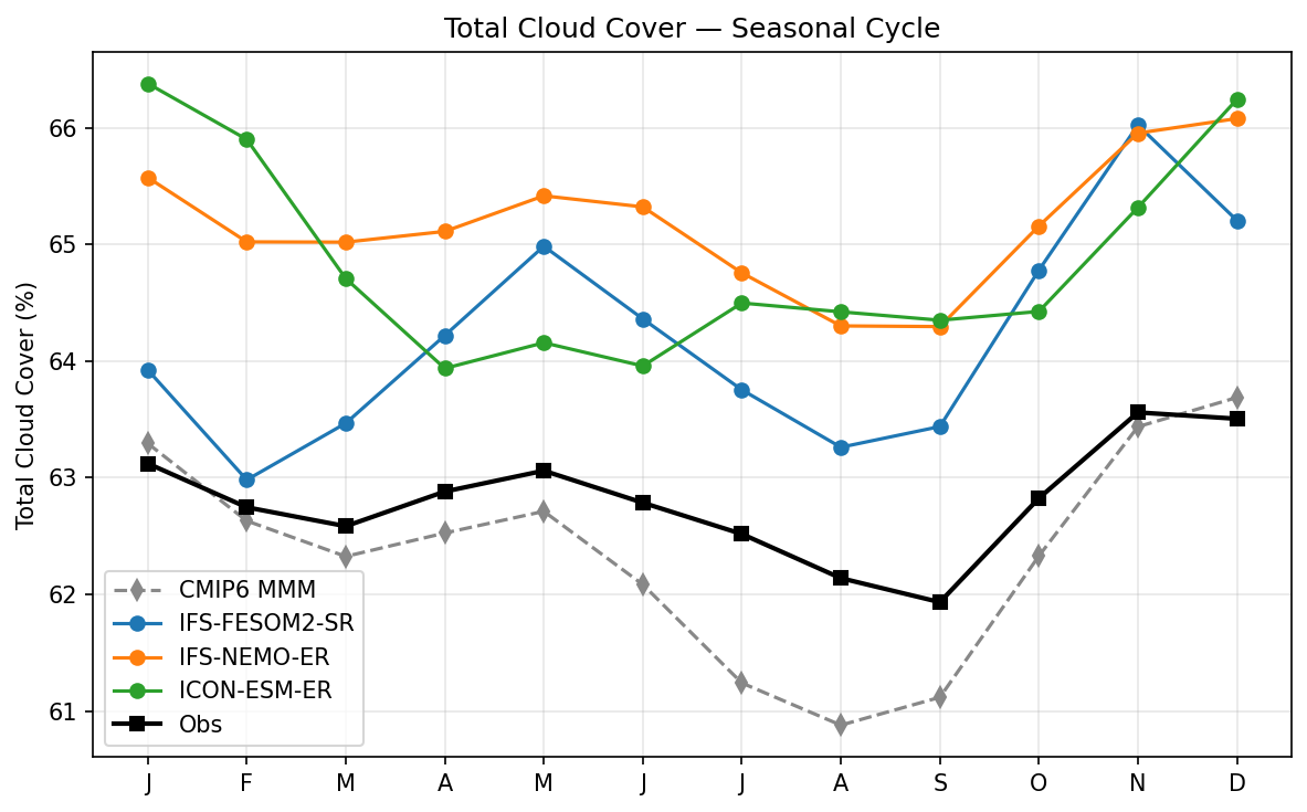
Total Cloud Cover Seasonal Cycle
| Variables | clt |
|---|---|
| Models | IFS-FESOM2-SR, IFS-NEMO-ER, ICON-ESM-ER |
| Reference Dataset | ERA5 |
| Units | % |
| Period | 1980–2014 |
Summary high
High-resolution models consistently overestimate global mean total cloud cover by 1–3% relative to ERA5 observations, whereas the CMIP6 multi-model mean tracks the observational magnitude and phase much more closely.
Key Findings
- All three evaluated high-resolution models (IFS-FESOM2-SR, IFS-NEMO-ER, ICON-ESM-ER) exhibit a systematic positive bias in total cloud cover (1–3% absolute) throughout the seasonal cycle compared to ERA5.
- The CMIP6 Multi-Model Mean provides the best agreement with observations, closely matching the ERA5 range (~62–63.5%) and seasonal phase, albeit with a slightly deeper minimum in August-September.
- ICON-ESM-ER displays the most pronounced seasonal amplitude, with a sharp, distinctive drop from January (~66.4%) to April (~64%) that is not present in the observations or other models.
- IFS-NEMO-ER maintains the highest sustained cloud cover among the models, rarely dropping below 64.5%.
Spatial Patterns
While this is a global-mean diagnostic, the temporal pattern shows a general seasonal minimum in boreal late summer (August-September) and a maximum in boreal winter (November-January) across observations and most models. ICON-ESM-ER deviates slightly with a very sharp early-year decline.
Model Agreement
There is a distinct separation between the high-resolution simulation group (biased high) and the CMIP6/Obs group (lower). Within the high-res group, the spread is roughly 1-2%, with IFS-FESOM2-SR generally being closest to observations and IFS-NEMO-ER/ICON-ESM-ER being cloudier.
Physical Interpretation
The systematic positive bias in the high-resolution models suggests either more vigorous convection or different cloud microphysics tuning compared to the standard resolution CMIP6 ensemble. Since ERA5 is generated using an older IFS cycle, the positive bias in IFS-FESOM/NEMO may reflect changes in model physics (e.g., cloud parametrization) or the lack of data assimilation in the free-running simulations allowing cloudiness to drift upwards. Excess cloud cover typically implies a bias towards stronger shortwave reflection (cooling), which impacts the Earth's radiation budget.
Caveats
- Global mean values can obscure compensating regional errors (e.g., excess tropical convection vs. deficit in stratocumulus decks).
- ERA5 is a reanalysis product and carries its own model biases, though it is constrained by observations.
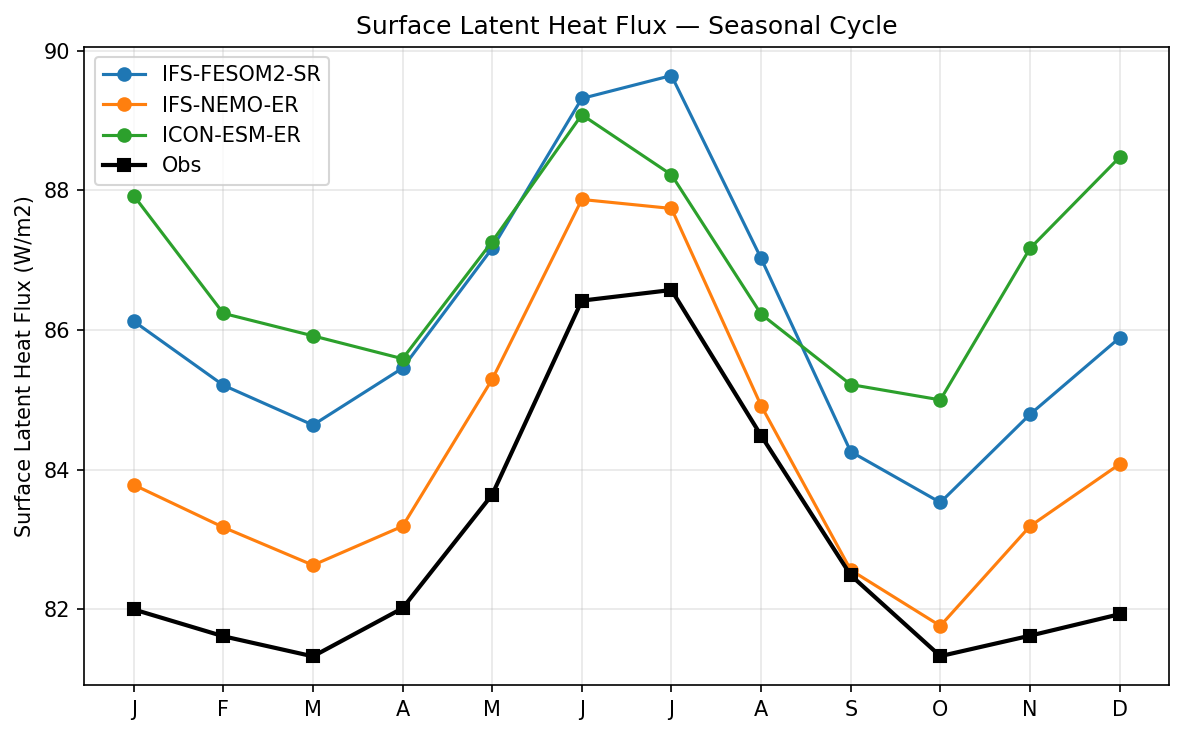
Surface Latent Heat Flux Seasonal Cycle
| Variables | hfls |
|---|---|
| Models | IFS-FESOM2-SR, IFS-NEMO-ER, ICON-ESM-ER |
| Reference Dataset | ERA5 |
| Units | W/m2 |
| Period | 1980–2014 |
Summary high
This figure displays the climatological seasonal cycle of global mean surface latent heat flux, comparing three high-resolution models against ERA5 reanalysis. All models consistently overestimate latent heat flux relative to ERA5, with IFS-NEMO-ER showing the best agreement and ICON-ESM-ER exhibiting the largest biases and a distorted seasonal shape.
Key Findings
- Systematic positive bias: All three models produce global mean latent heat fluxes higher than ERA5 throughout the entire year. Biases range from ~1.5 W/m² to >6 W/m² depending on the model and season.
- Best performer: IFS-NEMO-ER (orange) tracks the observational phase and amplitude most closely, with a relatively consistent positive offset of approximately 1–2 W/m².
- ICON-ESM-ER structural error: While capturing the mid-year peak, ICON-ESM-ER (green) shows excessively high fluxes in boreal winter (DJF), with values around 88 W/m² compared to the observational ~82 W/m², creating a spurious double-peak seasonal cycle.
- IFS-FESOM2-SR (blue) maintains the correct phase (peaking in July) but has a larger positive bias than the NEMO configuration, generally 2–4 W/m² higher than ERA5.
Spatial Patterns
The temporal cycle in observations shows a clear single peak in June-July (boreal summer), likely driven by evapotranspiration from the Northern Hemisphere land masses. The models generally reproduce this summer maximum, but the winter (DJF) period shows significant divergence, particularly with ICON's anomalously high values.
Model Agreement
There is good agreement on the timing of the primary maximum (June/July). However, inter-model spread is largest in boreal winter (Dec-Jan), where IFS-NEMO-ER remains close to the observational shape while ICON-ESM-ER diverges sharply.
Physical Interpretation
The universal positive bias suggests that these high-resolution models simulate excessive surface evaporation, which would act to cool the sea surface and inject excess moisture into the atmosphere, potentially driving an overly vigorous hydrological cycle (excess precipitation). ICON's specific winter bias points to potential issues with ocean surface turbulent flux parameterizations (bulk formulae) or excessive surface wind speeds over the oceans during winter, as global ocean evaporation typically dominates the winter signal.
Caveats
- Global means mask regional patterns; the positive bias could be spatially concentrated (e.g., in trade wind regions or western boundary currents).
- ERA5 fluxes are reanalysis products, meaning they are model-derived estimates constrained by observations, rather than direct measurements.
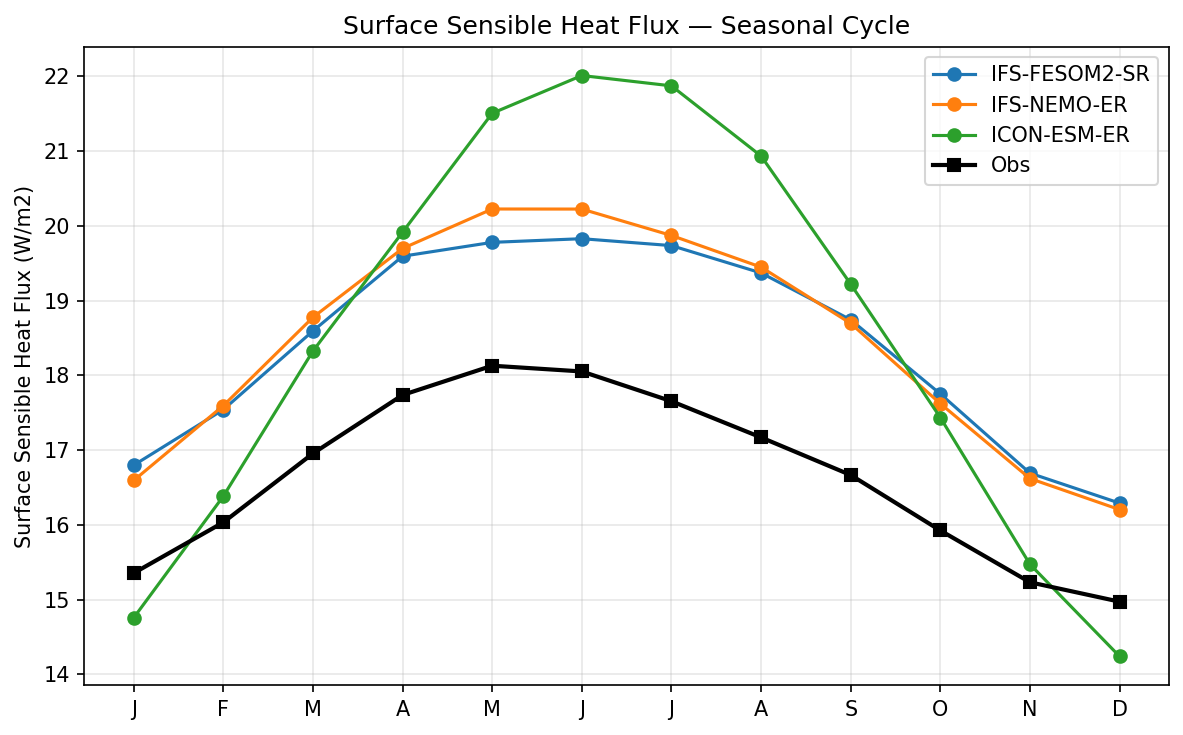
Surface Sensible Heat Flux Seasonal Cycle
| Variables | hfss |
|---|---|
| Models | IFS-FESOM2-SR, IFS-NEMO-ER, ICON-ESM-ER |
| Reference Dataset | ERA5 |
| Units | W/m2 |
| Period | 1980–2014 |
Summary high
The figure illustrates the global mean seasonal cycle of surface sensible heat flux (SHF) for three high-resolution climate models compared to ERA5 observations. While all models capture the phase of the cycle peaking in Northern Hemisphere summer, they exhibit distinct biases in magnitude and amplitude.
Key Findings
- All models generally overestimate the global mean sensible heat flux compared to the observational reference (ERA5), particularly during the Northern Hemisphere summer.
- IFS-FESOM2-SR and IFS-NEMO-ER track each other very closely with a consistent positive bias of ~1.5 to 2.5 W/m² throughout the year, suggesting the atmospheric component dictates this flux independent of the ocean model.
- ICON-ESM-ER exhibits a significantly amplified seasonal cycle, overestimating the summer peak by ~4 W/m² (reaching 22 W/m² vs ~18 W/m² in observations) while dipping slightly below observations in December/January.
Spatial Patterns
The seasonal cycle peaks in June-July, reflecting the dominance of Northern Hemisphere land masses where summer surface heating drives high sensible heat fluxes. ICON displays a much steeper spring rise (March-June) compared to the more gradual increase in the IFS models and observations.
Model Agreement
High agreement between the two IFS variants indicates robustness to ocean model choice. Significant disagreement exists between the IFS family and ICON regarding the cycle amplitude, with ICON showing much higher variance.
Physical Interpretation
Sensible heat flux is driven by the surface-to-air temperature gradient and turbulence. The systematic positive bias in IFS models suggests either consistently larger temperature gradients or more efficient transfer coefficients in the IFS physics package. The exaggerated amplitude in ICON-ESM-ER points to potential issues in the land-surface coupling, possibly excessive drying or heating of land surfaces in the NH summer, leading to overly strong fluxes.
Caveats
- The observational reference (ERA5) is a reanalysis product; sensible heat flux is a derived quantity dependent on the reanalysis model physics, not a direct observation.
- Global means effectively average over land (high seasonal cycle) and ocean (low seasonal cycle), obscuring potential regional compensating errors.
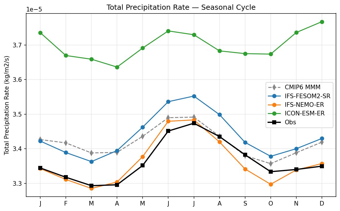
Total Precipitation Rate Seasonal Cycle
| Variables | pr |
|---|---|
| Models | IFS-FESOM2-SR, IFS-NEMO-ER, ICON-ESM-ER |
| Reference Dataset | ERA5 |
| Units | kg/m2/s |
| Period | 1980–2014 |
Summary high
This figure displays the seasonal cycle of global mean total precipitation rate, highlighting that IFS-NEMO-ER closely matches ERA5 reanalysis while ICON-ESM-ER and IFS-FESOM2-SR exhibit systematic wet biases.
Key Findings
- IFS-NEMO-ER demonstrates excellent agreement with ERA5 observations, accurately capturing both the absolute magnitude and the seasonal phase with minimal bias.
- ICON-ESM-ER exhibits a strong systematic positive (wet) bias, with global mean precipitation rates approximately 10% higher (~0.3-0.4e-5 kg/m²/s) than observations throughout the year.
- IFS-FESOM2-SR and the CMIP6 Multi-Model Mean (MMM) share a moderate positive bias relative to ERA5, with IFS-FESOM2-SR tracking the CMIP6 MMM closely.
Spatial Patterns
All datasets show a consistent seasonal phase driven by planetary geometry and land distribution: a global minimum in March/April and a maximum in July/August (boreal summer). This peak corresponds to the seasonal northward shift of the ITCZ and the dominance of Northern Hemisphere monsoon precipitation over larger land masses.
Model Agreement
There is strong inter-model disagreement regarding the mean magnitude of the hydrological cycle. IFS-NEMO-ER agrees best with observations. ICON-ESM-ER is a distinct outlier with the highest precipitation rates. IFS-FESOM2-SR aligns with the typical biases seen in the CMIP6 ensemble.
Physical Interpretation
The wet bias in ICON-ESM-ER and IFS-FESOM2-SR suggests an overly active global hydrological cycle, likely driven by excessive global surface evaporation or atmospheric radiative cooling constraints that require balancing latent heat release. The close match of IFS-NEMO-ER to ERA5 suggests its eddy-rich ocean coupling or tuning effectively constrains global energy and moisture budgets.
Caveats
- The observational reference is ERA5 (reanalysis), which itself may contain biases compared to satellite/gauge products like GPCP, particularly in the tropics.
- Global mean precipitation is an energetic constraint; discrepancies may stem from offsetting errors in radiative fluxes rather than just microphysics.
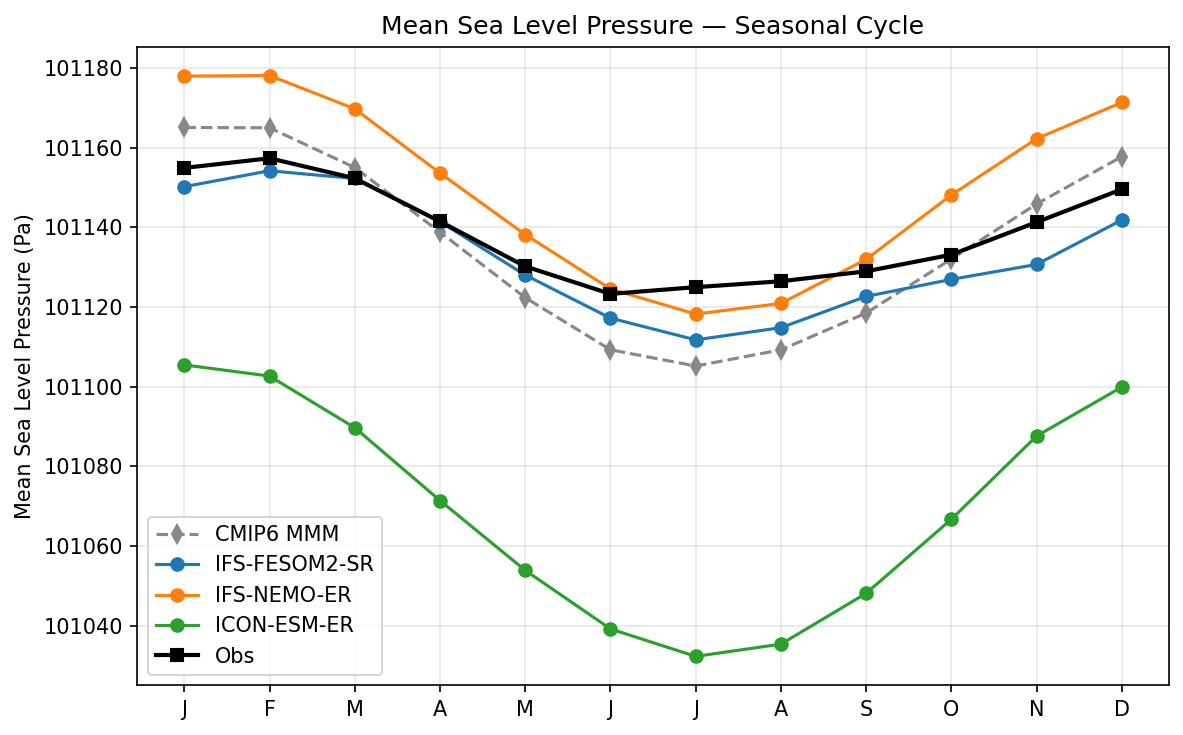
Mean Sea Level Pressure Seasonal Cycle
| Variables | psl |
|---|---|
| Models | IFS-FESOM2-SR, IFS-NEMO-ER, ICON-ESM-ER |
| Reference Dataset | ERA5 |
| Units | Pa |
| Period | 1980–2014 |
Summary high
The figure illustrates the seasonal cycle of global mean Mean Sea Level Pressure (MSLP), revealing significant systematic offsets in total atmospheric mass or pressure reduction between the models despite good agreement on the seasonal phase.
Key Findings
- ICON-ESM-ER exhibits a large, systematic negative bias of approximately 80-100 Pa (~1 hPa) relative to ERA5 throughout the annual cycle.
- IFS-NEMO-ER shows a consistent positive bias of roughly 20-30 Pa, while IFS-FESOM2-SR tracks closest to observations, showing a small negative bias (<10 Pa).
- All models and the CMIP6 MMM correctly capture the phase of the seasonal cycle, with a global minimum in boreal summer (June-July) and maximum in boreal winter (December-January).
- The CMIP6 Multi-Model Mean exaggerates the amplitude of the seasonal cycle, with a deeper minimum in summer compared to ERA5 and the high-resolution IFS models.
Spatial Patterns
While this is a global-mean time series, the temporal pattern shows a distinct seasonal cycle driven by Northern Hemisphere land-sea thermal contrasts. The global mean MSLP is lowest in JJA, consistent with the 'thermal low' effect where reduction to sea level under warm conditions over large NH landmasses results in lower calculated pressures.
Model Agreement
There is strong agreement on the phase of the seasonal cycle across all datasets. However, there is significant disagreement on the absolute magnitude (the global mean state), with a spread of nearly 1.5 hPa between the highest (IFS-NEMO-ER) and lowest (ICON-ESM-ER) models. IFS-FESOM2-SR provides the best match to the ERA5 amplitude and mean state.
Physical Interpretation
The seasonal variation is primarily an artifact of the mathematical reduction of surface pressure to sea level; warmer temperatures in the NH summer (dominated by land) lead to lower reduced pressures (thermal lows). The constant offsets between models likely stem from differences in the total atmospheric mass initialization or conservation (tuning of the dry air mass) rather than dynamical feedback errors. The slight difference between IFS-NEMO and IFS-FESOM (which share the same atmosphere) implies influence from the underlying ocean/ice state or coupling frequency on the global pressure integration or water vapor loading.
Caveats
- Global mean MSLP is a calculated quantity dependent on reduction algorithms over topography, not a direct measurement of total atmospheric mass (which is Surface Pressure).
- The large bias in ICON may be a static initialization offset rather than a process drift.
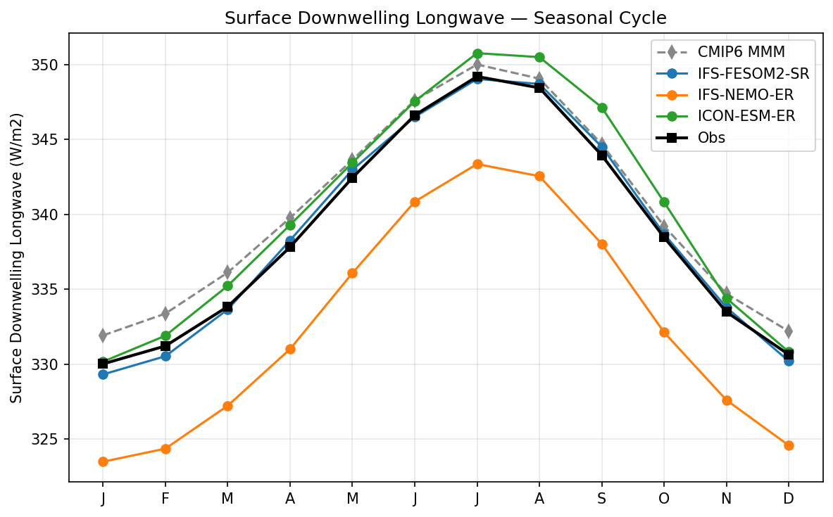
Surface Downwelling Longwave Seasonal Cycle
| Variables | rlds |
|---|---|
| Models | IFS-FESOM2-SR, IFS-NEMO-ER, ICON-ESM-ER |
| Reference Dataset | ERA5 |
| Units | W/m2 |
| Period | 1980–2014 |
Summary high
This figure displays the global mean seasonal cycle of surface downwelling longwave radiation ($rlds$) for three EERIE models and the CMIP6 multi-model mean compared against ERA5 reanalysis.
Key Findings
- IFS-FESOM2-SR demonstrates exceptional agreement with ERA5 observations, tracking the seasonal amplitude and magnitude almost perfectly throughout the year.
- IFS-NEMO-ER exhibits a substantial systematic negative bias of approximately 6-7 W/m² year-round, despite correctly capturing the phase of the seasonal cycle.
- ICON-ESM-ER shows a moderate positive bias (~1-2 W/m²), particularly during boreal summer and autumn (July–October), closely resembling the behavior of the CMIP6 Multi-Model Mean.
- All models correctly reproduce the seasonal phase, with a global maximum in July/August driven by the dominance of Northern Hemisphere landmasses and summer temperatures.
Spatial Patterns
The seasonal cycle is characterized by a minimum in January (~324-332 W/m²) and a maximum in July (~343-350 W/m²). The global mean signal is dominated by the Northern Hemisphere seasonal cycle.
Model Agreement
Inter-model agreement is poor regarding magnitude. There is a large spread (~7-8 W/m²) between the lowest model (IFS-NEMO-ER) and the highest (ICON-ESM-ER/CMIP6). IFS-FESOM2-SR is the distinct 'best performer' relative to the ERA5 reference.
Physical Interpretation
Surface downwelling longwave radiation is primarily controlled by near-surface air temperature, specific humidity (water vapor), and cloud cover. The large negative bias in IFS-NEMO-ER suggests a global cold/dry bias in the lower troposphere or insufficient cloudiness compared to ERA5. Conversely, the positive bias in ICON-ESM-ER and CMIP6 suggests a slightly too warm/moist atmosphere or excessive cloud radiative effect. The stark difference between IFS-NEMO-ER and IFS-FESOM2-SR (which share an atmospheric core but differ in ocean coupling/resolution) points to significant sensitivity of the boundary layer thermodynamics to the specific model configuration (SR vs ER) or ocean state.
Caveats
- The observational reference is ERA5 reanalysis, which, while a standard benchmark for surface fields, is model-derived; comparisons with direct CERES surface products might yield slight differences.
- The cause of the IFS-NEMO-ER bias (atmosphere vs. ocean driven) cannot be fully isolated without complementary SST or humidity bias plots.
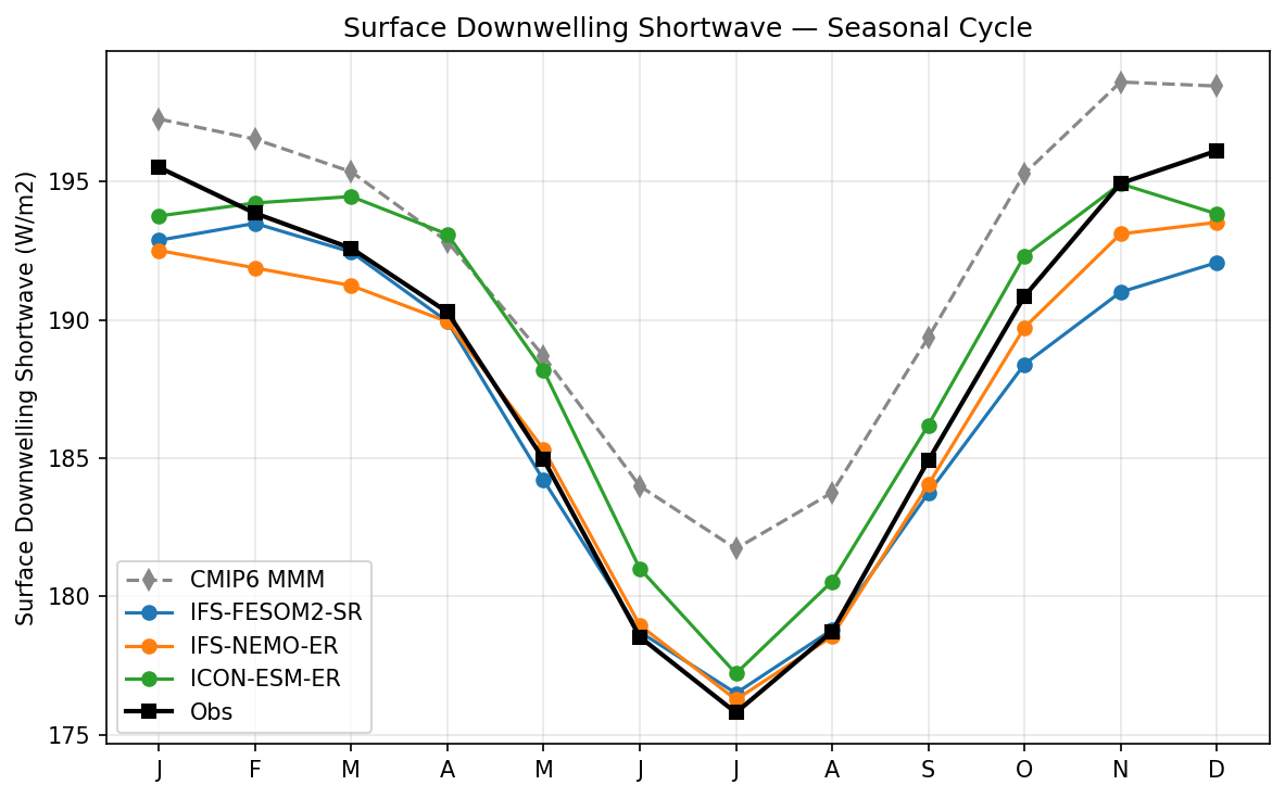
Surface Downwelling Shortwave Seasonal Cycle
| Variables | rsds |
|---|---|
| Models | IFS-FESOM2-SR, IFS-NEMO-ER, ICON-ESM-ER |
| Reference Dataset | ERA5 |
| Units | W/m2 |
| Period | 1980–2014 |
Summary high
This figure displays the seasonal cycle of global mean surface downwelling shortwave radiation (rsds), revealing that the high-resolution EERIE models (especially IFS variants) align much more closely with ERA5 observations than the CMIP6 Multi-Model Mean.
Key Findings
- The CMIP6 Multi-Model Mean (MMM) exhibits a systematic positive bias of approximately 3–6 W/m² throughout the year compared to ERA5 observations.
- IFS-NEMO-ER demonstrates the strongest agreement with observations, closely tracking the ERA5 seasonal cycle with deviations generally under 1 W/m².
- ICON-ESM-ER shows a positive bias relative to observations during transition months (March-May and October-November) but aligns well during the solstice months.
- The seasonal amplitude (January maximum vs. July minimum) is accurately captured by the EERIE models (~19 W/m² range), whereas the CMIP6 MMM shows a damped amplitude (~16 W/m²).
Spatial Patterns
The temporal pattern follows the Earth's orbital eccentricity, with maximum global insolation near perihelion (January) and minimum near aphelion (July).
Model Agreement
High-resolution models cluster closer to observations than the coarse-resolution CMIP6 ensemble. Within the EERIE group, IFS-NEMO-ER and IFS-FESOM2-SR show high consistency in summer but diverge slightly in winter, while ICON-ESM-ER is an outlier with higher values in spring/autumn.
Physical Interpretation
The pervasive positive bias in CMIP6 suggests an underestimation of atmospheric attenuation (likely due to insufficient cloud cover or optical thickness), leading to excessive solar radiation reaching the surface. The EERIE models appear to correct this 'surface brightening' bias, potentially due to improved cloud parameterizations or resolution-dependent dynamics. The seasonal cycle itself is driven by the variation in solar distance.
Caveats
- Global averaging masks potential regional compensating errors (e.g., biases in specific cloud regimes).
- The observational reference is ERA5 reanalysis; comparisons with direct satellite products (like CERES) would validate the reanalysis accuracy.
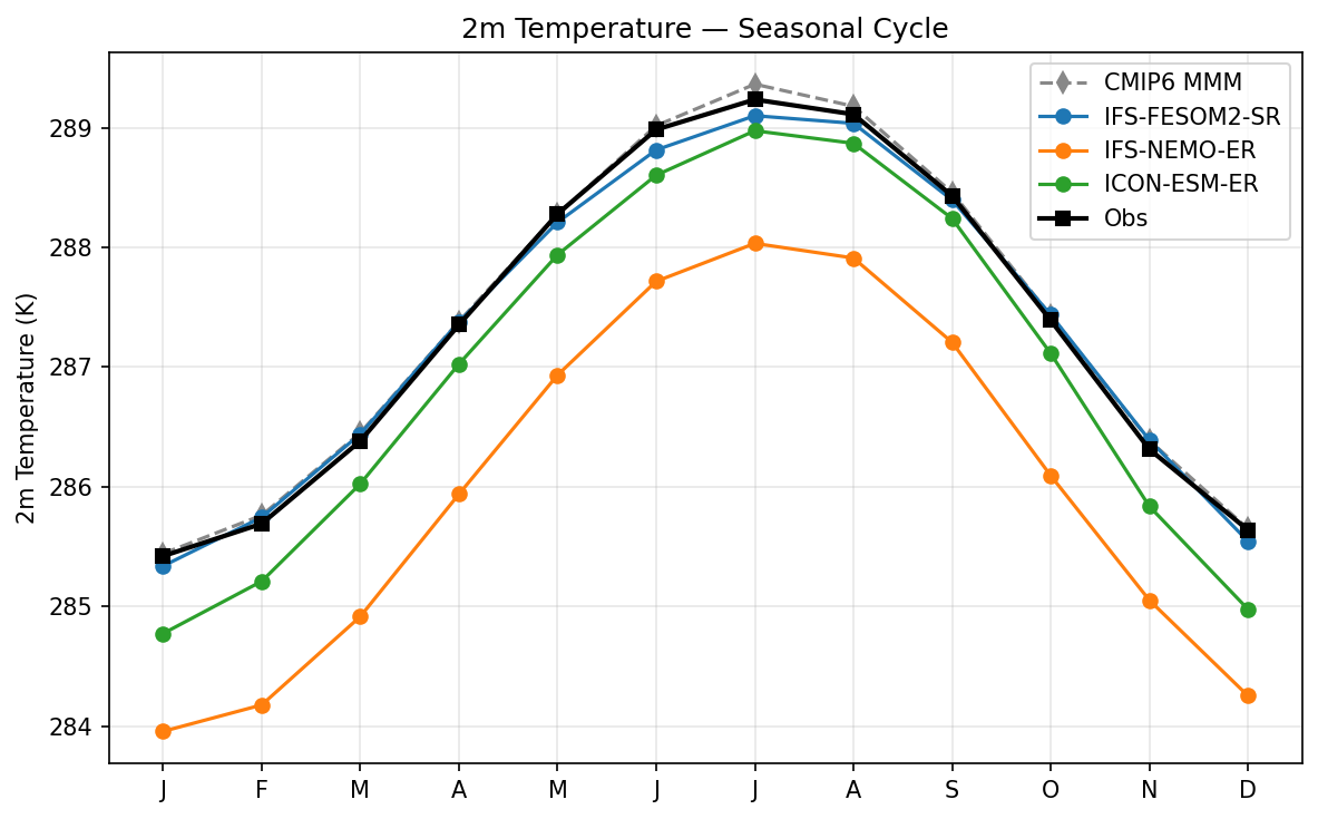
2m Temperature Seasonal Cycle
| Variables | tas |
|---|---|
| Models | IFS-FESOM2-SR, IFS-NEMO-ER, ICON-ESM-ER |
| Reference Dataset | ERA5 |
| Units | K |
| Period | 1980–2014 |
Summary high
This figure compares the seasonal cycle of global mean 2-meter temperature from three high-resolution EERIE models against ERA5 observations and the CMIP6 multi-model mean.
Key Findings
- IFS-FESOM2-SR shows remarkable agreement with ERA5 observations, tracking the seasonal evolution almost perfectly with negligible bias (< 0.1 K in most months).
- IFS-NEMO-ER exhibits a severe systematic cold bias of approximately 1.5 K throughout the entire year, representing the largest deviation among the evaluated models.
- ICON-ESM-ER displays a consistent cold bias of roughly 0.5–0.6 K relative to observations, maintaining the correct phase and amplitude but shifted to lower temperatures.
- The CMIP6 Multi-Model Mean tracks observations closely, with a slight warm bias (~0.1 K) evident during the boreal summer peak (July-August).
Spatial Patterns
While spatial patterns are not shown, the temporal seasonal cycle peaks in July (~289.3 K in observations) and reaches a minimum in January (~285.4 K), reflecting the dominance of Northern Hemisphere landmass thermal inertia.
Model Agreement
There is strong agreement on the phase and amplitude of the seasonal cycle (approximately 4 K range) across all models, indicating correct representation of first-order seasonal drivers. However, there is significant disagreement in the absolute mean state, particularly for IFS-NEMO-ER.
Physical Interpretation
The correct phase across all models confirms they capture the hemispheric asymmetry of land-mass heating. The large cold bias in IFS-NEMO-ER compared to IFS-FESOM2-SR (which shares the same atmospheric component) strongly implicates the NEMO ocean configuration or the coupling strategy (e.g., sea surface temperature biases or sea ice extent) as the primary driver of the global mean temperature deficit.
Caveats
- Global mean metrics may mask compensating regional biases (e.g., warm biases in one region offsetting cold biases elsewhere).
- The cause of the IFS-NEMO-ER cold bias cannot be fully diagnosed without inspecting SST and sea ice spatial maps.
10m U Wind Seasonal Cycle
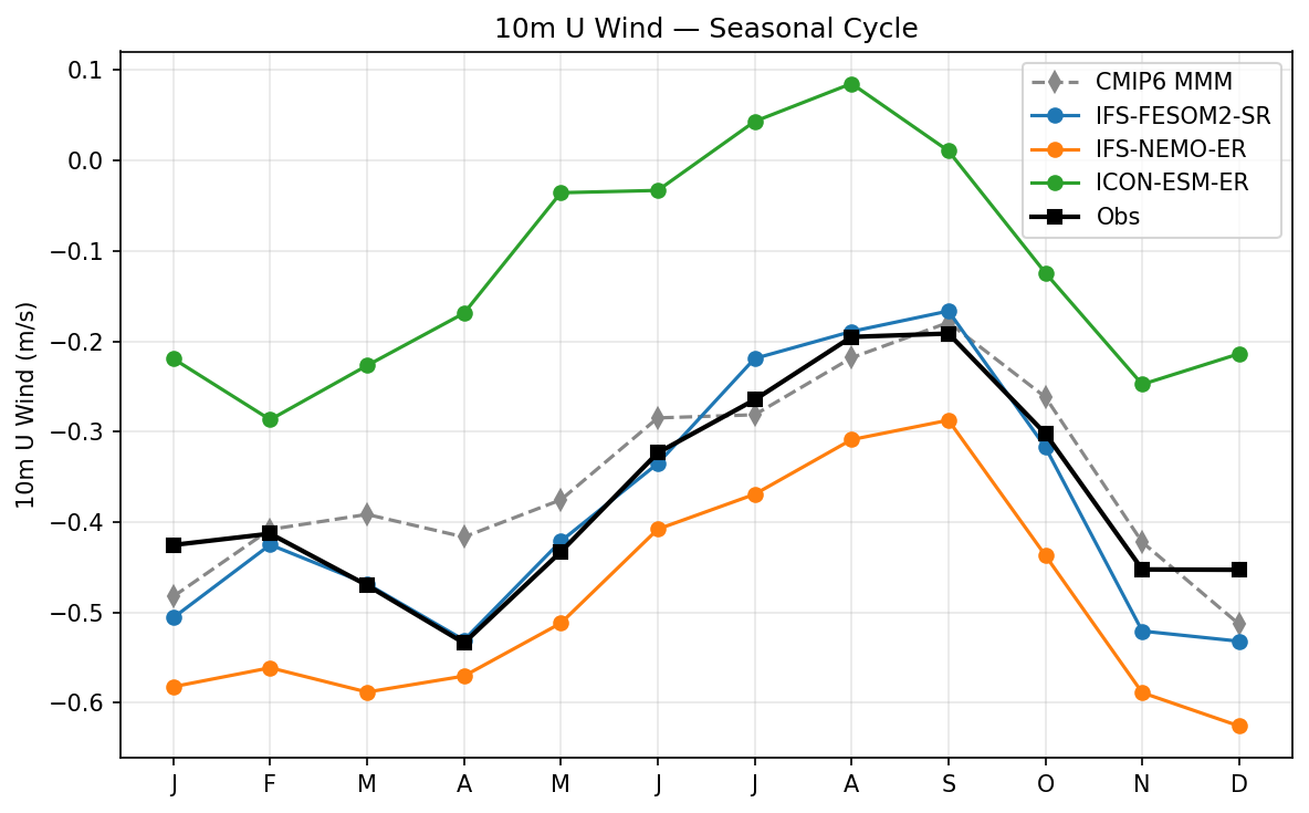
| Variables | uas |
|---|---|
| Models | IFS-FESOM2-SR, IFS-NEMO-ER, ICON-ESM-ER |
| Reference Dataset | ERA5 |
| Units | m/s |
| Period | 1980–2014 |
Summary high
This figure illustrates the global mean 10m zonal (U) wind seasonal cycle, highlighting significant mean-state biases between models despite good phase agreement.
Key Findings
- IFS-FESOM2-SR shows exceptional agreement with ERA5 observations, tracking the seasonal cycle phase and magnitude almost perfectly and outperforming the CMIP6 multi-model mean.
- IFS-NEMO-ER exhibits a systematic negative bias of approximately -0.15 m/s (stronger easterly mean) relative to observations, despite sharing the same atmospheric component as IFS-FESOM.
- ICON-ESM-ER displays a large positive bias (~+0.25 m/s), erroneously simulating a net westerly global mean wind during boreal summer (June-September), contradicting the easterly mean seen in observations.
- All models correctly capture the seasonal phase, with a minimum (strongest easterlies) in April and a maximum (weakest easterlies) in September.
Spatial Patterns
The temporal evolution shows a clear seasonal cycle with an amplitude of ~0.35 m/s. The global mean is consistently negative (easterly) in observations, driven by the extensive tropical trade wind belts. ICON is the only model to cross into positive (westerly) global mean values during boreal summer.
Model Agreement
While phase agreement is high, inter-model agreement on magnitude is poor. The spread between models (~0.5 m/s) exceeds the amplitude of the seasonal cycle itself, indicating significant uncertainty in the global mean surface wind balance.
Physical Interpretation
The negative global mean U-wind reflects the dominance of trade wind surface area over mid-latitude westerlies. The stark difference between IFS-FESOM and IFS-NEMO (which share the IFS atmosphere) strongly suggests that air-sea coupling differences—specifically how SSTs or surface currents feed back into stability-dependent drag coefficient calculations—are driving the mean state offsets. ICON's positive bias implies potential issues with weak trade winds or overly strong mid-latitude westerlies.
Caveats
- Global mean values can mask compensating regional errors (e.g., overly strong NH westerlies balancing weak SH westerlies).
- Analysis of 10m winds depends on the specific surface layer parameterization used to interpolate from the lowest model level.
10m V Wind Seasonal Cycle
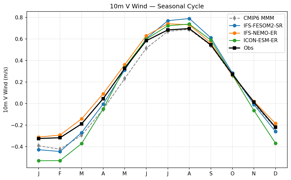
| Variables | vas |
|---|---|
| Models | IFS-FESOM2-SR, IFS-NEMO-ER, ICON-ESM-ER |
| Reference Dataset | ERA5 |
| Units | m/s |
| Period | 1980–2014 |
Summary high
The figure illustrates the seasonal cycle of global mean 10m meridional (V) wind, comparing three high-resolution models against ERA5 observations and the CMIP6 multi-model mean. While all models capture the fundamental phase driven by the seasonal migration of the Intertropical Convergence Zone (ITCZ), significant differences appear in the amplitude of the cycle.
Key Findings
- ICON-ESM-ER exhibits a distinct negative bias during boreal winter (Dec-Feb), showing excessive global southward flow (~-0.55 m/s vs -0.33 m/s in observations).
- IFS-FESOM2-SR overamplifies the seasonal cycle, producing a deeper trough in winter and a higher peak in summer compared to ERA5.
- IFS-NEMO-ER shows the best agreement with observations, tracking the ERA5 winter minimum closely, though slightly overestimating the boreal summer peak.
- The CMIP6 multi-model mean generally underestimates the amplitude of the cycle, particularly the rate of increase in northward flow during boreal spring (May-June), whereas the high-resolution models capture this transition more sharply.
Spatial Patterns
The seasonal cycle follows the global atmospheric circulation shift: net southward surface flow in boreal winter (negative V) and net northward flow in boreal summer (positive V), peaking in July-August due to cross-equatorial flows like the Asian Monsoon.
Model Agreement
Inter-model spread is largest in boreal winter (Jan-Mar) and late autumn (Nov-Dec), with ICON-ESM-ER acting as a negative outlier. In boreal summer (JJA), models cluster more closely around the observational peak (~0.7 m/s), though all tend to slightly overshoot the ERA5 maximum.
Physical Interpretation
Global mean V-wind is a residual quantity reflecting hemispheric asymmetries in Hadley cell strength and cross-equatorial flow (e.g., monsoons). Positive values indicate net northward flow (JJA), and negative values indicate net southward flow (DJF). The strong negative bias in ICON during DJF suggests overly strong Northern Hemisphere trade winds or enhanced southward cross-equatorial transport compared to observations.
Caveats
- Global mean meridional wind is a small residual of large opposing fluxes; seemingly small biases here can imply significant regional circulation errors.
- The analysis does not isolate specific regions (e.g., tropics vs mid-latitudes), so the source of the global bias (e.g., monsoon strength vs mid-latitude storm tracks) cannot be pinpointed without spatial maps.