Evaluation Climate Variability Modes CMIP6
CMIP6 Multi-Model Mean Context
Comparison with CMIP6 ensemble mean from 11 members.
Contributing models: ACCESS-ESM1-5, AWI-CM-1-1-MR, CNRM-CM6-1, CNRM-ESM2-1, EC-Earth3, FGOALS-g3, GISS-E2-1-G, INM-CM5-0, IPSL-CM6A-LR, MPI-ESM1-2-LR, MRI-ESM2-0
Synthesis
Related diagnostics
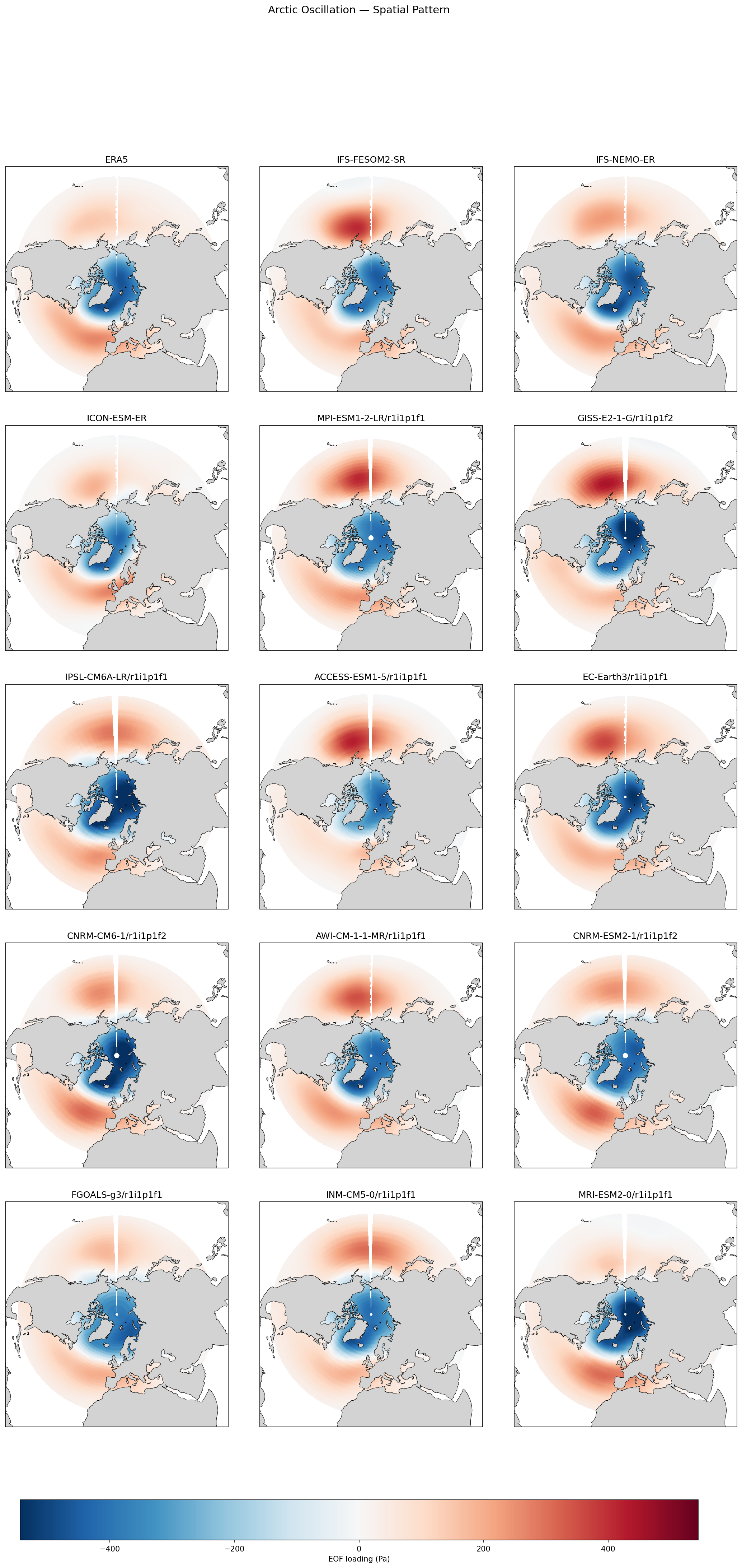
Arctic Oscillation — Spatial Pattern
| Variables | psl |
|---|---|
| Models | IFS-FESOM2-SR, IFS-NEMO-ER, ICON-ESM-ER |
| Reference Dataset | ERA5 |
| Units | Pa |
| Period | 1980–2014 |
| IFS-FESOM2-SR | Variance Explained: 0.21 |
| IFS-NEMO-ER | Variance Explained: 0.22 |
| ICON-ESM-ER | Variance Explained: 0.15 |
| ERA5 | Variance Explained: 0.20 |
Summary high
This figure illustrates the spatial structure of the Arctic Oscillation (AO), derived as the leading EOF of sea level pressure (psl), comparing ERA5 reanalysis with three high-resolution EERIE models and a selection of CMIP6 models.
Key Findings
- IFS-FESOM2-SR and IFS-NEMO-ER show excellent skill in reproducing the AO spatial pattern, capturing the characteristic negative pressure anomaly over the Arctic and positive anomalies over the North Atlantic and North Pacific.
- The variance explained by the AO in IFS-FESOM2-SR (20.9%) and IFS-NEMO-ER (22.4%) is consistent with, or slightly higher than, ERA5 (19.9%), indicating realistic amplitude of variability.
- ICON-ESM-ER significantly underestimates the AO strength and variance explained (14.9%), with a notably washed-out pattern and a particularly weak center of action over the North Pacific.
- Compared to the CMIP6 ensemble, the IFS models perform among the best, avoiding the over-amplified Pacific centers seen in models like MPI-ESM1-2-LR or the weak patterns in INM-CM5-0.
Spatial Patterns
The dominant pattern is the classic annular mode: a deep negative loading centered over the Arctic Ocean/Greenland (blue) surrounded by a ring of positive loading in the mid-latitudes (red). Two distinct mid-latitude centers of action are visible in the North Atlantic and North Pacific sectors.
Model Agreement
There is high agreement between ERA5 and the two IFS-based models regarding pattern shape and magnitude. ICON-ESM-ER diverges by showing much weaker coupling between the Arctic and the North Pacific sector. The CMIP6 models show a spread in the relative strength of the Pacific vs. Atlantic centers, with most capturing the gross features.
Physical Interpretation
The AO represents the fluctuating exchange of atmospheric mass between the Arctic and mid-latitudes, modulating the strength of the westerly polar vortex. The weak Pacific center in ICON-ESM-ER suggests a decoupling of the Aleutian Low variability from the hemispheric annular mode or errors in the Pacific mean state/storm track dynamics. The robust performance of IFS suggests that increasing resolution (SR/ER) preserves or enhances the representation of these large-scale dynamical modes.
Caveats
- The sign of EOF patterns is arbitrary; patterns have been oriented to show the positive phase (low Arctic pressure) for consistency.
- Comparison relies on EOF1, assuming the AO is the leading mode in all models (variance explained confirms it is, though lower in ICON).
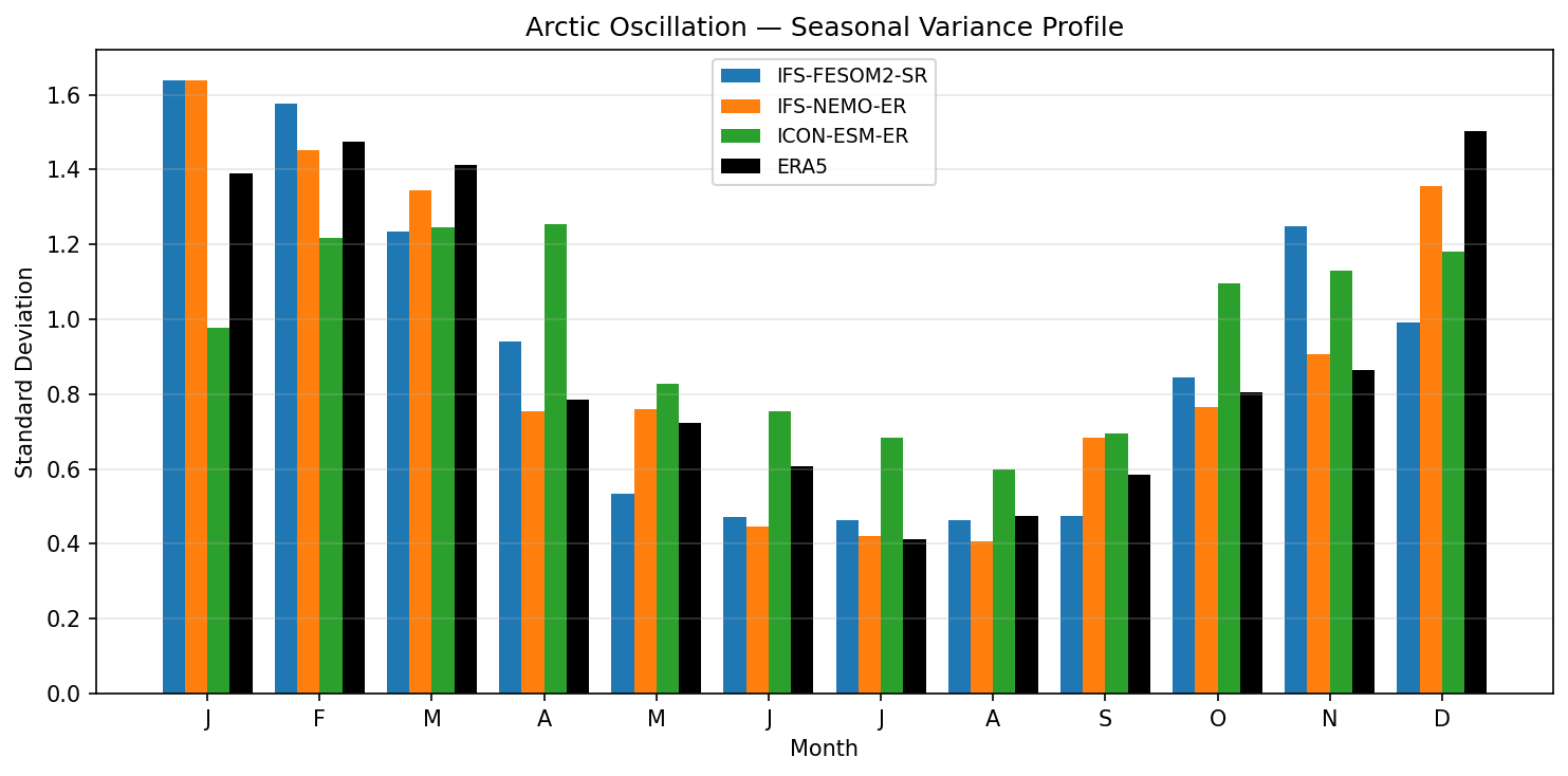
Arctic Oscillation — Seasonal Variance Profile
| Variables | psl |
|---|---|
| Models | IFS-FESOM2-SR, IFS-NEMO-ER, ICON-ESM-ER |
| Reference Dataset | ERA5 |
| Units | Pa |
| Period | 1980–2014 |
| IFS-FESOM2-SR | Peak Month: 1.00 · Peak Std: 1.64 · Annual Std: 1.00 |
| IFS-NEMO-ER | Peak Month: 1.00 · Peak Std: 1.64 · Annual Std: 1.00 |
| ICON-ESM-ER | Peak Month: 4.00 · Peak Std: 1.25 · Annual Std: 1.00 |
Summary high
This figure evaluates the seasonal cycle of Arctic Oscillation (AO) variability across three high-resolution coupled models compared to ERA5, illustrating distinct performance differences between the IFS and ICON model families.
Key Findings
- ERA5 displays the expected AO seasonal cycle: dominant variability in winter (DJF, std ~1.4–1.5) and a minimum in summer (JJA, std ~0.4).
- Both IFS-based models (IFS-FESOM2-SR and IFS-NEMO-ER) capture the correct seasonal phase but overestimate winter variability, particularly in January and February (std > 1.6).
- ICON-ESM-ER fails to reproduce the observed seasonal structure, underestimating winter variability and producing a spurious variance peak in April alongside systematic overestimation of summer and autumn variability.
Spatial Patterns
The observation and IFS models show a U-shaped seasonal profile (high winter, low summer). In contrast, ICON-ESM-ER exhibits a much flatter profile with a physically unrealistic mid-spring maximum (April) and fails to achieve the quiescent summer state observed in ERA5.
Model Agreement
The two IFS models agree closely with each other, suggesting the atmospheric component dominates the AO signal regardless of the ocean coupling (FESOM2 vs NEMO). ICON-ESM-ER diverges significantly from both the IFS models and observations.
Physical Interpretation
The AO is dynamically driven by tropospheric eddy-mean flow interactions and stratospheric coupling, which are most active in boreal winter. The IFS models capture this vigorous winter dynamics, albeit with excessive amplitude, potentially implying too strong a jet or stratospheric vortex variability. ICON's dampened winter and anomalous spring/summer activity suggest a fundamental bias in its representation of the Northern Hemisphere background circulation and seasonal modulation of storm tracks.
Caveats
- The indices are likely normalized over the full time series (annual std = 1.0), so seasonal deviations represent the redistribution of variance throughout the year.
- The spurious April peak in ICON requires further investigation into potential biases in spring sea-ice retreat or stratospheric final warming timing.
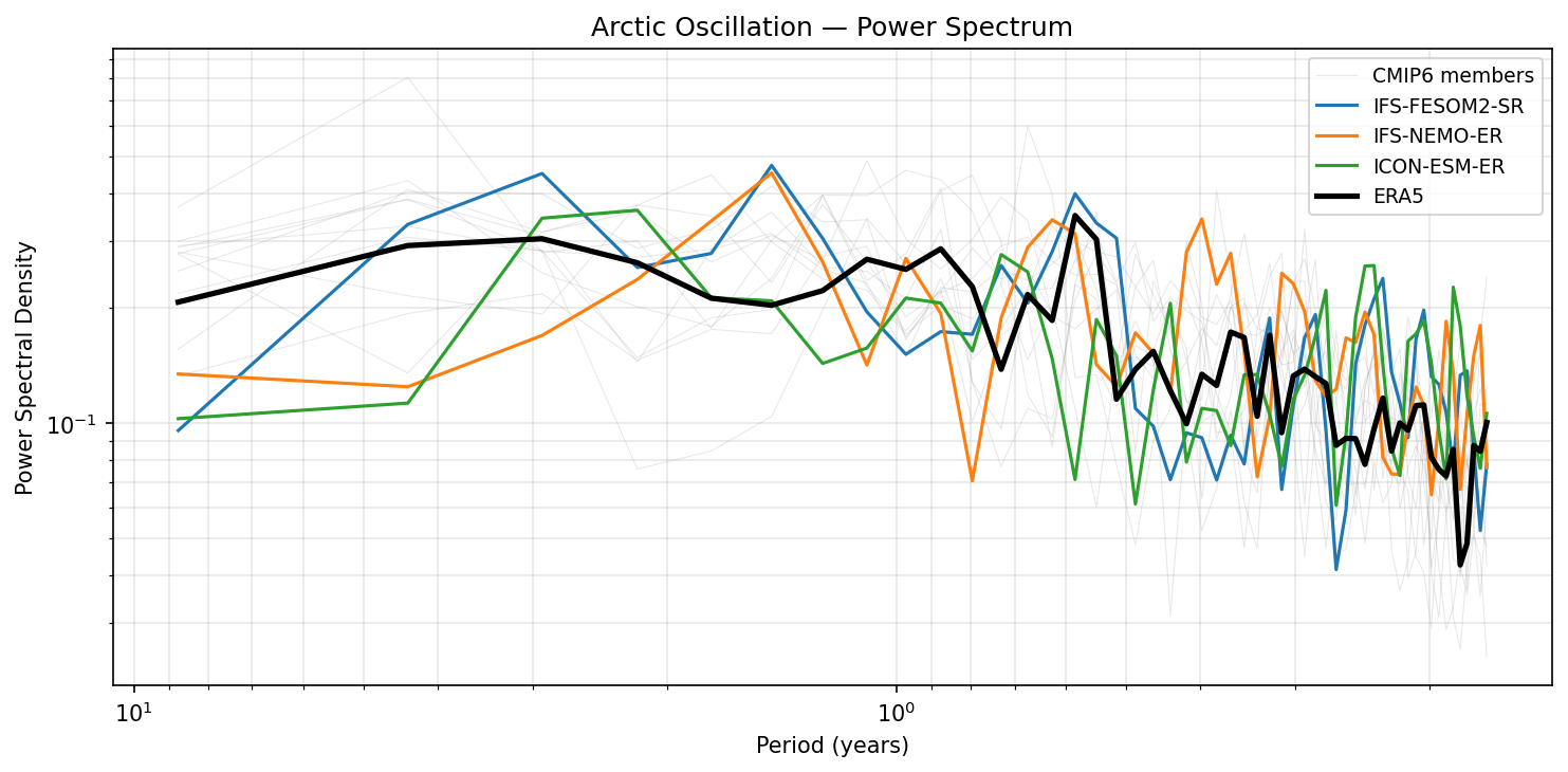
Arctic Oscillation — Power Spectrum
| Variables | psl |
|---|---|
| Models | IFS-FESOM2-SR, IFS-NEMO-ER, ICON-ESM-ER |
| Reference Dataset | ERA5 |
| Units | Pa |
| Period | 1980–2014 |
Summary high
This spectral analysis compares the variability of the Arctic Oscillation (AO) index in three high-resolution coupled models against ERA5 reanalysis and the CMIP6 ensemble over the 1980–2014 period. The models generally reproduce the observed spectral shape, but significant differences emerge in variability amplitude at interannual to decadal timescales.
Key Findings
- IFS-FESOM2-SR reproduces the decadal-scale (>5 years) power density of ERA5 remarkably well, whereas IFS-NEMO-ER and ICON-ESM-ER underestimate variability in this low-frequency band.
- In the interannual band (2–5 years), both IFS-based models (FESOM and NEMO) exhibit distinct spectral peaks that exceed the power found in ERA5, which shows a flatter plateau in this range.
- At sub-annual periods (<1 year), all three models closely track the ERA5 power spectrum and fall well within the CMIP6 ensemble spread, indicating a realistic representation of high-frequency atmospheric stochastic variability.
- ICON-ESM-ER consistently shows the lowest power spectral density across the interannual to decadal range, often tracking the lower bound of the CMIP6 ensemble spread.
Spatial Patterns
N/A (Temporal frequency analysis). The general pattern is a 'red' spectrum with power increasing at longer periods, consistent with theoretical expectations for the AO.
Model Agreement
Agreement is high at high frequencies (sub-annual) where all models converge with observations. Divergence increases significantly at low frequencies (>2 years), with IFS-FESOM2-SR aligning best with observations and ICON-ESM-ER showing the weakest low-frequency variability.
Physical Interpretation
The AO spectrum typically follows a red noise profile, resulting from the integration of stochastic atmospheric forcing. The divergence between IFS-FESOM2-SR and IFS-NEMO-ER (which share the same IFS atmospheric component) at low frequencies suggests that differences in ocean/sea-ice models or coupling strategies may influence the long-term persistence (memory) of the oscillation, although internal variability plays a strong role.
Caveats
- The analysis period (1980–2014) is relatively short (35 years), making the estimation of decadal spectral power statistically uncertain (few degrees of freedom).
- Differences between single model realizations at low frequencies may reflect internal variability rather than systematic physics biases, as indicated by the wide spread of the CMIP6 background ensemble.
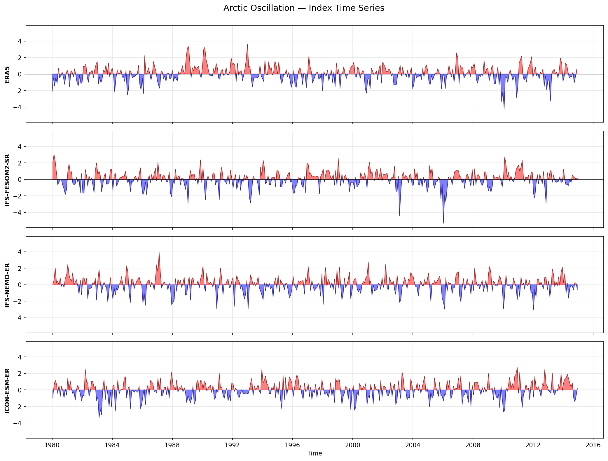
Arctic Oscillation — Index Time Series
| Variables | psl |
|---|---|
| Models | IFS-FESOM2-SR, IFS-NEMO-ER, ICON-ESM-ER |
| Reference Dataset | ERA5 |
| Units | Pa |
| Period | 1980–2014 |
| IFS-FESOM2-SR | Std: 1.00 · Mean: 0.00 |
| IFS-NEMO-ER | Std: 1.00 · Mean: 0.00 |
| ICON-ESM-ER | Std: 1.00 · Mean: 0.00 |
Summary high
This figure presents the monthly time series of the standardized Arctic Oscillation (AO) index for the period 1980–2014, comparing ERA5 reanalysis against three high-resolution coupled climate models (IFS-FESOM2-SR, IFS-NEMO-ER, ICON-ESM-ER).
Key Findings
- All evaluated models successfully reproduce the stochastic variability and dynamic range of the observed Arctic Oscillation, with index values typically fluctuating within ±2 standard deviations and occasionally reaching extremes of ±4.
- The models exhibit the capability to simulate extreme AO phases comparable to observations; for instance, IFS-FESOM2-SR produces a negative excursion exceeding -4 sigma (resembling the ERA5 2010 event magnitude), while IFS-NEMO-ER produces a positive excursion exceeding +4 sigma.
- As expected for free-running coupled simulations, the specific timing of AO phases does not match the historical ERA5 record (e.g., the deep 2009/2010 negative phase), but the statistical character of the time series is consistent with observations.
Spatial Patterns
The time series are characterized by 'red noise' variability typical of atmospheric teleconnections, with no obvious unrealistic drifts, periodicities, or trends visible in the model outputs over the 35-year period.
Model Agreement
There is strong statistical agreement between the models and ERA5 regarding the amplitude and frequency of AO fluctuations. The standardization (std=1.0) confirms that the leading modes of variability in the models account for a comparable proportion of variance to reality.
Physical Interpretation
The Arctic Oscillation represents the vacillation of atmospheric mass between the Arctic and mid-latitudes, driven by internal dynamics of the jet stream and storm tracks. The realistic index behavior indicates that the high-resolution models (10 km atmosphere) adequately resolve the eddy-mean flow interactions and Rossby wave breaking processes that sustain this annular mode.
Caveats
- Direct correlation of event timing is not expected as these are un-nudged historical simulations.
- Without power spectra, it is difficult to assess if the models capture the correct persistence timescales (e.g., stratosphere-troposphere coupling timescales).
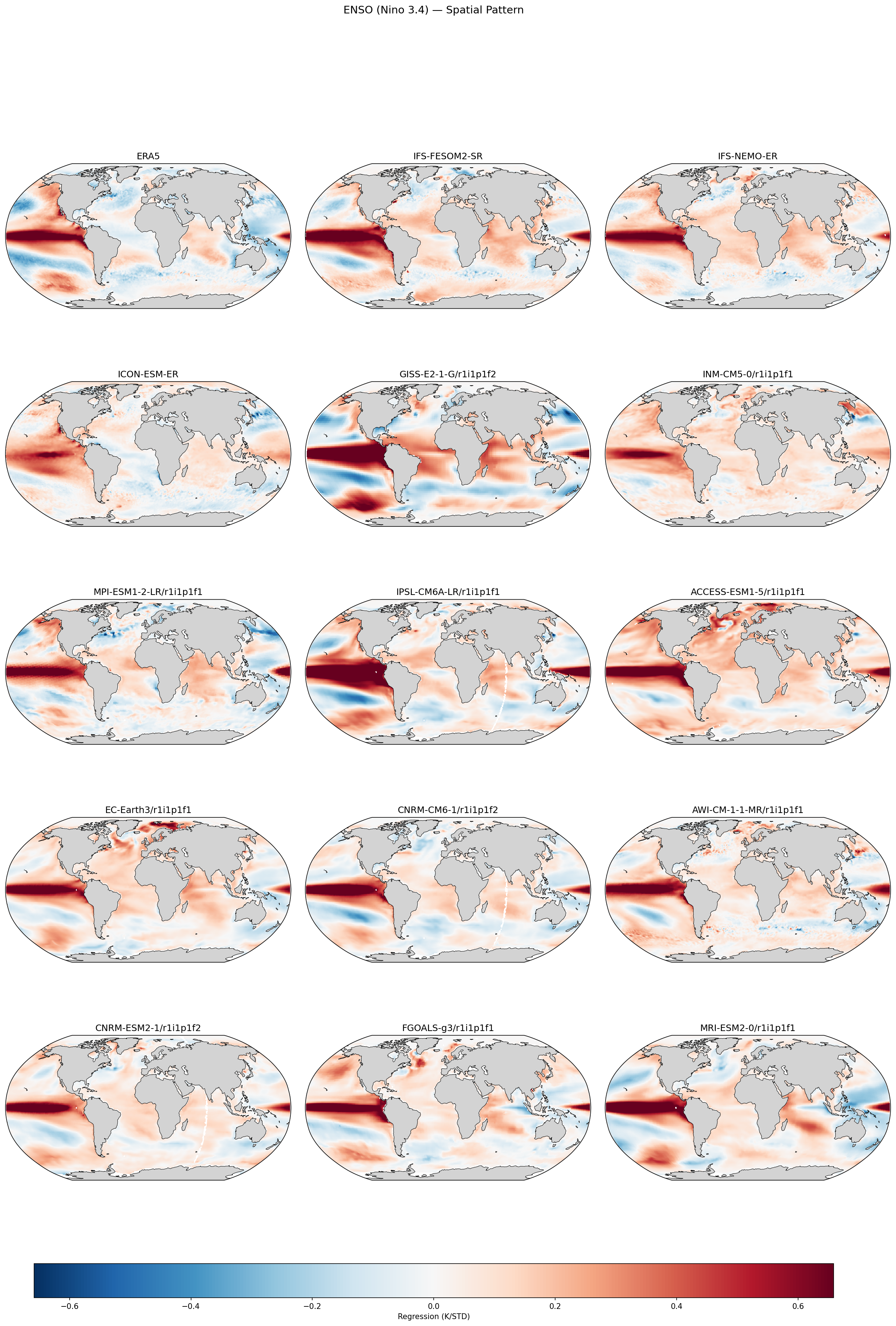
ENSO (Nino 3.4) — Spatial Pattern
| Variables | tos |
|---|---|
| Models | IFS-FESOM2-SR, IFS-NEMO-ER, ICON-ESM-ER |
| Reference Dataset | ESA_CCI |
| Units | K |
| Period | 1980–2014 |
Summary high
The diagnostic evaluates the spatial pattern of ENSO (SST regression onto Niño 3.4 index) in high-resolution EERIE models compared to ERA5 and a CMIP6 ensemble. The EERIE models generally reproduce the canonical tongue structure and meridional confinement well, though with variations in the longitudinal extent of the warming signal.
Key Findings
- IFS-FESOM2-SR and IFS-NEMO-ER exhibit robust ENSO spatial patterns with realistic meridional confinement of equatorial anomalies, outperforming lower-resolution CMIP6 outliers like GISS-E2-1-G which show excessive meridional spread.
- IFS-FESOM2-SR displays a westward bias in the extension of the equatorial warming tongue, with positive anomalies penetrating deeper into the western Pacific warm pool compared to ERA5 and IFS-NEMO-ER.
- IFS-NEMO-ER captures the transition to negative anomalies (the western Pacific horseshoe) more accurately than IFS-FESOM2-SR, aligning closely with the ERA5 reference.
- Global teleconnections, such as the Indian Ocean Basin Mode warming and the North Pacific PDO-like pattern, are well-captured by the high-resolution IFS models.
Spatial Patterns
The classic ENSO pattern—an elongated tongue of warming in the central/eastern equatorial Pacific flanked by a horseshoe of cooling in the west—is visible in the reference. EERIE models capture the basin-wide Indian Ocean warming response and the off-equatorial Pacific anomalies.
Model Agreement
There is high agreement between the high-resolution IFS models and the better-performing CMIP6 models (e.g., EC-Earth3, MRI-ESM2-0). However, the CMIP6 ensemble shows significant spread in pattern fidelity (e.g., GISS-E2-1-G is too broad; INM-CM5-0 is too weak), highlighting the value of the higher-resolution simulations.
Physical Interpretation
The spatial pattern reflects the Bjerknes feedback mechanism, where trade wind relaxation reinforces SST warming. The meridional confinement in high-resolution models suggests better resolved equatorial waveguide dynamics (Kelvin/Rossby waves). The westward shift in IFS-FESOM2-SR suggests a bias in the mean state cold tongue boundary or trade wind stress fetch.
Caveats
- The plot shows regression coefficients (K/STD), essentially normalizing the pattern amplitude; this does not show if the absolute variance of ENSO (amplitude in K) is correct.
- The reference is labelled ERA5 but metadata states ESA_CCI; since ERA5 assimilates SST, they are effectively consistent, but this distinction is noted.
ENSO (Nino 3.4) — Seasonal Variance Profile
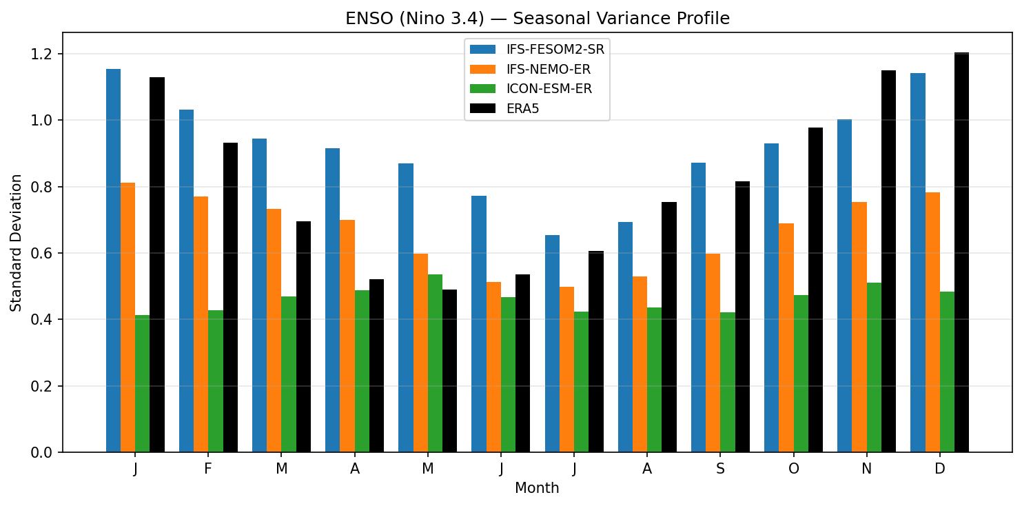
| Variables | tos |
|---|---|
| Models | IFS-FESOM2-SR, IFS-NEMO-ER, ICON-ESM-ER |
| Reference Dataset | ESA_CCI |
| Units | K |
| Period | 1980–2014 |
| IFS-FESOM2-SR | Peak Month: 1.00 · Peak Std: 1.15 · Annual Std: 0.93 |
| IFS-NEMO-ER | Peak Month: 1.00 · Peak Std: 0.81 · Annual Std: 0.67 |
| ICON-ESM-ER | Peak Month: 5.00 · Peak Std: 0.54 · Annual Std: 0.46 |
Summary high
This figure evaluates the seasonal variance profile of the ENSO (Nino 3.4) index, revealing that IFS-FESOM2-SR accurately reproduces the observed amplitude and seasonal phase locking, whereas IFS-NEMO-ER and ICON-ESM-ER significantly underestimate variability.
Key Findings
- ERA5 observations (black) show the characteristic ENSO seasonal cycle: peak variance in boreal winter (DJF, std > 1.1 K) and a minimum in late spring/early summer (May-July, std ~0.5-0.6 K).
- IFS-FESOM2-SR (blue) shows excellent agreement with ERA5, matching both the magnitude of the winter peak (~1.15 K) and the timing of the seasonal minimum.
- IFS-NEMO-ER (orange) captures the correct seasonal phase (peaking in DJF) but systematically underestimates the amplitude by approximately 30-40% across all months.
- ICON-ESM-ER (green) fails to capture ENSO variability, showing a flat, weak profile (std ~0.4-0.5 K) with no distinct winter peak, effectively missing the seasonal phase locking.
Spatial Patterns
The temporal pattern highlights the 'spring predictability barrier' in observations (variance minimum in MJJ) and the phase locking of mature ENSO events to the boreal winter (DJF). Only IFS-FESOM2-SR faithfully replicates this strong seasonality.
Model Agreement
There is strong inter-model divergence. IFS-FESOM2-SR is the only model that aligns with the observational baseline (ERA5). IFS-NEMO-ER shows moderate skill in phase but weak amplitude, while ICON-ESM-ER exhibits very poor skill with drastically suppressed tropical variability.
Physical Interpretation
The realistic variance in IFS-FESOM2-SR suggests well-resolved Bjerknes feedback mechanisms (coupling between SST, wind stress, and thermocline depth). The weak variability in IFS-NEMO-ER and ICON-ESM-ER implies either overly strong damping fluxes, errors in the mean state (e.g., cold tongue bias) suppressing convection, or insufficient air-sea coupling strength to sustain ENSO growth.
Caveats
- The analysis is limited to SST variance (Nino 3.4) and does not diagnose the specific coupled feedback components (e.g., thermocline or wind stress feedbacks) causing the suppression in ICON and IFS-NEMO.
ENSO (Nino 3.4) — Power Spectrum
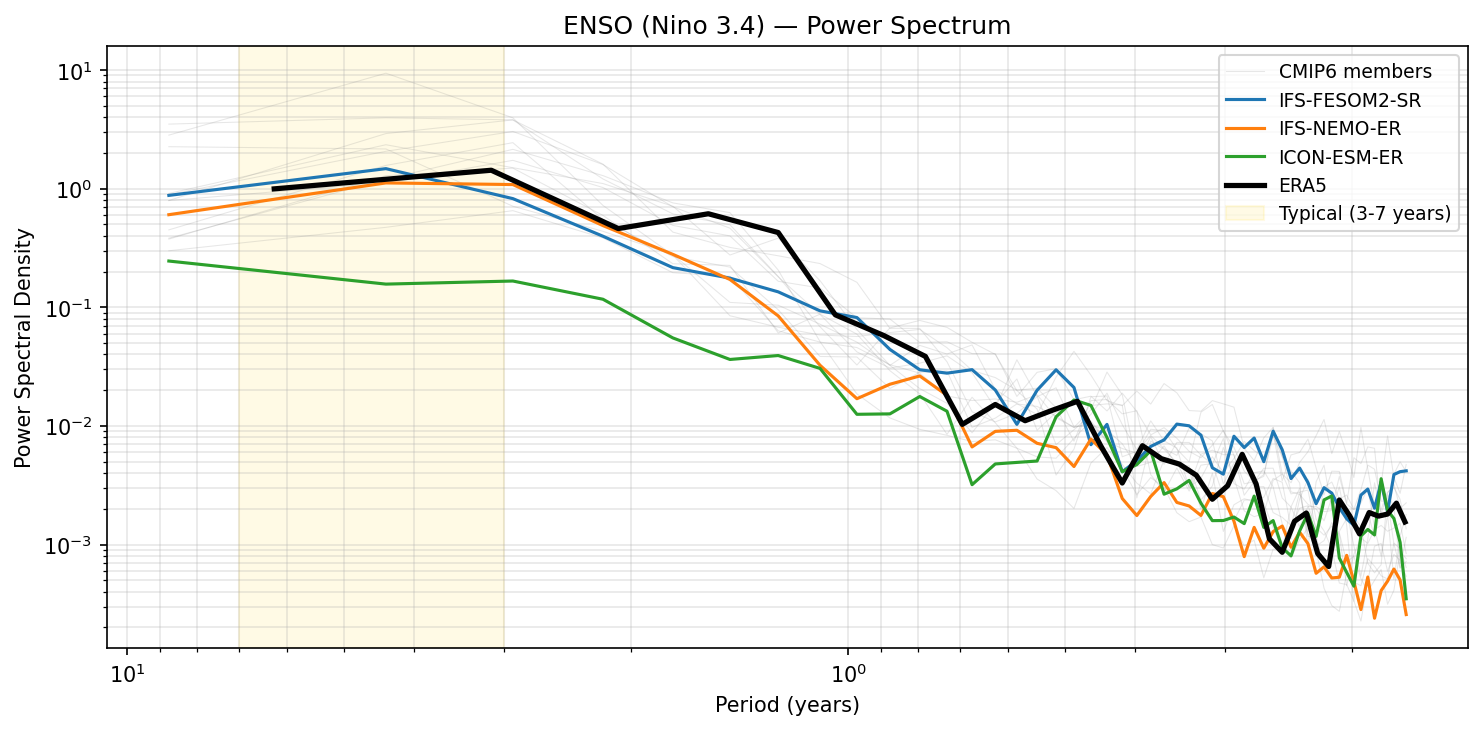
| Variables | tos |
|---|---|
| Models | IFS-FESOM2-SR, IFS-NEMO-ER, ICON-ESM-ER |
| Reference Dataset | ESA_CCI |
| Units | K |
| Period | 1980–2014 |
Summary high
This spectral analysis of the Niño 3.4 index demonstrates that the IFS-based models successfully reproduce the observed ENSO periodicity, while ICON-ESM-ER fails to generate significant interannual variability.
Key Findings
- IFS-FESOM2-SR and IFS-NEMO-ER show power spectra that align well with ERA5 and the CMIP6 ensemble, capturing the distinct spectral peak in the 3-7 year band.
- ICON-ESM-ER exhibits severely suppressed variability, with power spectral density nearly an order of magnitude lower than observations in the critical 3-7 year range.
- IFS-FESOM2-SR shows slightly higher high-frequency energy (<1 year period) compared to IFS-NEMO-ER and ERA5.
Spatial Patterns
N/A (Spectral analysis). The dominant variability in observations and IFS models is correctly concentrated in the interannual band (3-7 years), typical of ENSO dynamics.
Model Agreement
High agreement between IFS variants and ERA5. ICON-ESM-ER is a significant outlier, falling well below the envelope of CMIP6 members.
Physical Interpretation
The realistic spectra in IFS models suggest effective Bjerknes feedback and ocean-atmosphere coupling. The flat, low-power spectrum in ICON-ESM-ER indicates that the coupled system is overly damped or lacks the necessary feedbacks to sustain the ENSO oscillation, resulting in variability closer to white noise than a coherent mode.
Caveats
- The analysis period (1980-2014) is relatively short for resolving decadal modulation of ENSO spectral peaks.
- Spectral analysis alone does not diagnose the phase or spatial structure of the events, only their frequency and amplitude.
ENSO (Nino 3.4) — Index Time Series
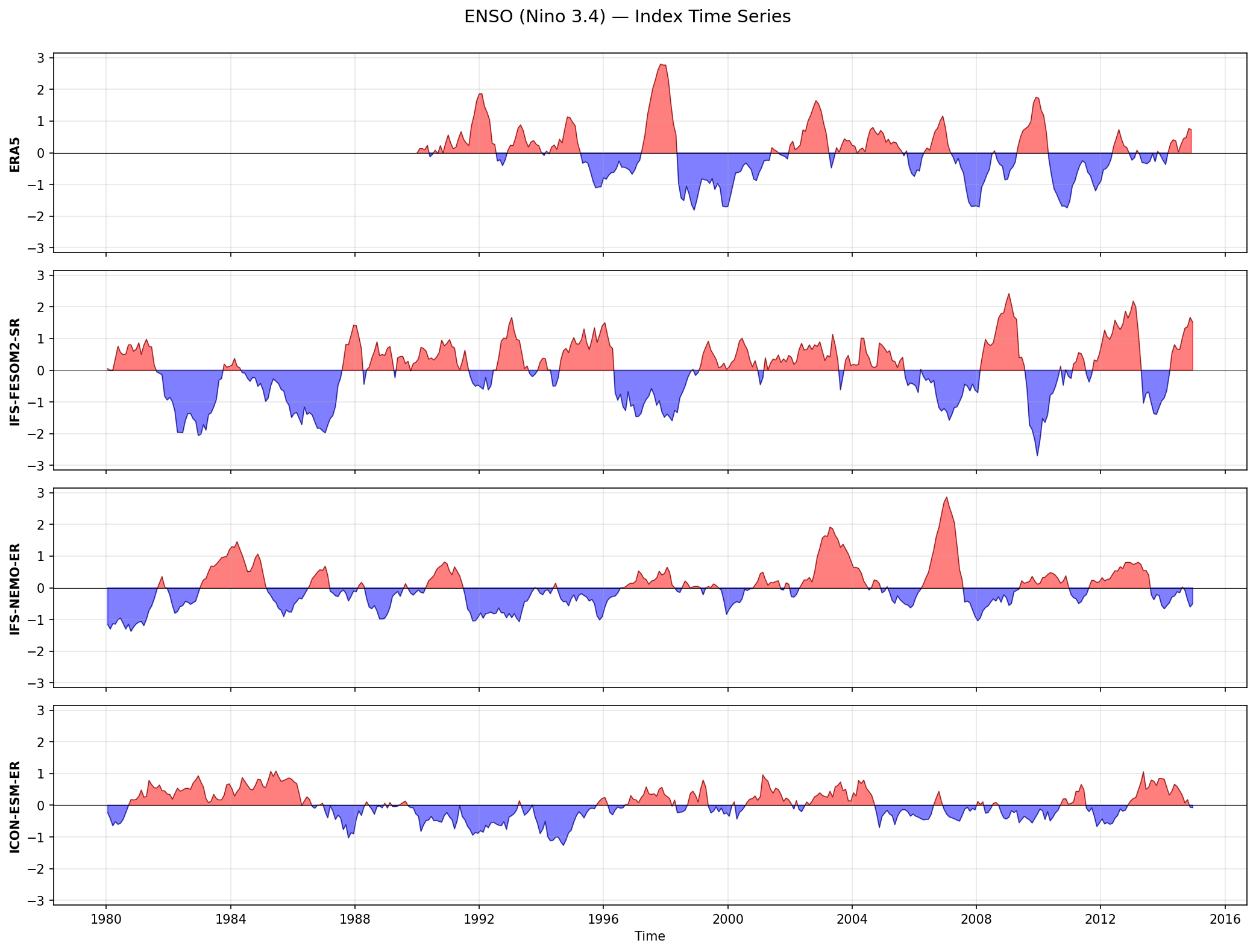
| Variables | tos |
|---|---|
| Models | IFS-FESOM2-SR, IFS-NEMO-ER, ICON-ESM-ER |
| Reference Dataset | ESA_CCI |
| Units | K |
| Period | 1980–2014 |
| IFS-FESOM2-SR | Std: 0.93 · Mean: -0.00 |
| IFS-NEMO-ER | Std: 0.67 · Mean: 0.00 |
| ICON-ESM-ER | Std: 0.46 · Mean: 0.00 |
Summary high
This figure shows the time series of the Nino 3.4 sea surface temperature anomaly index for ERA5 reanalysis and three high-resolution coupled models. There is a stark divergence in simulated ENSO amplitude, ranging from realistic variability in IFS-FESOM2-SR to a strongly damped cycle in ICON-ESM-ER.
Key Findings
- IFS-FESOM2-SR exhibits the most robust ENSO variability (std ~0.93 K), producing high-amplitude events (>2 K) that compare well with the magnitude of historical extremes like the 1997/98 El Niño.
- ICON-ESM-ER suffers from a severe 'weak ENSO' bias (std ~0.46 K), with anomalies rarely exceeding 1 K and lacking distinct strong El Niño or La Niña events.
- IFS-NEMO-ER shows intermediate variability (std ~0.67 K), generally underestimating the variance seen in IFS-FESOM2-SR and observations, though it is capable of producing isolated strong events.
- The observational panel (ERA5) displays the characteristic irregular 3-7 year cycle with peaks exceeding 2.5 K, which is best mimicked by the IFS-FESOM2-SR configuration.
Spatial Patterns
N/A (Time series analysis). The temporal structure in ERA5 clearly identifies historical events (1982/83, 1997/98, 2015/16), while model time series show uncorrelated internal variability as expected from free-running simulations.
Model Agreement
Models disagree significantly on ENSO amplitude. IFS-FESOM2-SR and IFS-NEMO-ER (sharing the same atmospheric component) diverge notably, with FESOM producing ~40% higher standard deviation than NEMO.
Physical Interpretation
The large difference between IFS-FESOM2-SR and IFS-NEMO-ER implies that the ocean model formulation (unstructured FESOM vs structured NEMO) is the primary driver of the amplitude differences, likely via differences in numerical mixing, thermocline sharpness, or resolution of Tropical Instability Waves (TIWs). The muted variability in ICON-ESM-ER suggests a weak Bjerknes feedback loop, possibly due to a too-diffuse thermocline or weak wind-SST coupling, preventing the growth of anomalies.
Caveats
- The 35-year analysis period is relatively short for robustly characterizing ENSO statistics, which exhibit multi-decadal modulation.
- Models are free-running, so event timing is not expected to match observations; evaluation is based purely on statistical properties (amplitude, frequency).
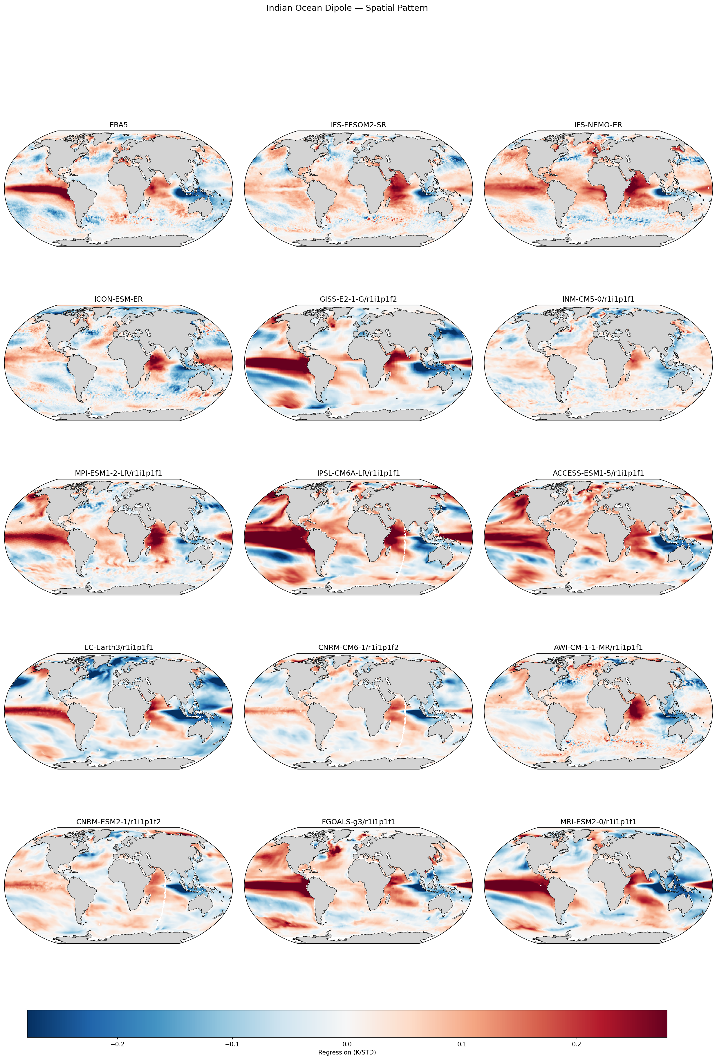
Indian Ocean Dipole — Spatial Pattern
| Variables | tos |
|---|---|
| Models | IFS-FESOM2-SR, IFS-NEMO-ER, ICON-ESM-ER |
| Reference Dataset | ESA_CCI |
| Units | K |
| Period | 1980–2014 |
Summary high
This figure illustrates the spatial sea surface temperature (SST) patterns associated with the Indian Ocean Dipole (IOD) in high-resolution EERIE models compared to ERA5/ESA-CCI and a suite of CMIP6 models. The analysis focuses on the fidelity of the zonal dipole mode within the Indian Ocean and its teleconnection to the Pacific (ENSO).
Key Findings
- High-resolution models (IFS-NEMO-ER, IFS-FESOM2-SR, ICON-ESM-ER) accurately reproduce the canonical IOD pattern, with well-defined cooling off Sumatra/Java and warming in the western Indian Ocean, matching the spatial structure of ERA5.
- There is significant inter-model spread in the teleconnection to the Pacific Ocean (ENSO linkage). IFS-NEMO-ER closely matches the ERA5 pattern showing a distinct El Niño-like signature, whereas IFS-FESOM2-SR shows a much weaker Pacific response, implying weaker ENSO-IOD coupling.
- Many CMIP6 models (e.g., IPSL-CM6A-LR, MRI-ESM2-0) exhibit excessively strong regression coefficients in the tropical Pacific compared to ERA5, suggesting that IOD variability in these models may be too strongly driven by ENSO rather than internal dynamics.
Spatial Patterns
The observed pattern (ERA5) is characterized by a sharp negative SST anomaly in the eastern Indian Ocean (coastal upwelling region) and a broader positive anomaly in the west. A positive tongue of warming extends into the central/eastern Pacific, reflecting the statistical association between the positive IOD and El Niño. The high-resolution models generally capture the coastal confinement of the eastern pole better than coarser CMIP6 models (e.g., GISS-E2-1-G, INM-CM5-0), which tend to produce more diffuse anomalies.
Model Agreement
The three EERIE high-resolution models agree well on the Indian Ocean dipole structure itself. However, they diverge on the global teleconnection footprint. IFS-NEMO-ER demonstrates the best agreement with ERA5 regarding the magnitude and spatial extent of the associated Pacific and Atlantic signals. ICON-ESM-ER also performs well but with slightly patchier Pacific signals. IFS-FESOM2-SR produces a more spatially isolated Indian Ocean signal.
Physical Interpretation
The core pattern is driven by the Bjerknes feedback within the Indian Ocean (coupling between zonal winds and SST gradients). The Pacific signal represents the 'atmospheric bridge' where ENSO-induced Walker circulation shifts trigger IOD events. Models with overpowering Pacific signals (many CMIP6) likely overestimate this external forcing or have overly energetic ENSO modes. The weaker Pacific link in IFS-FESOM2-SR suggests it may generate IOD events more independently of ENSO compared to IFS-NEMO-ER.
Caveats
- The reference panel is labelled 'ERA5' but metadata indicates 'ESA_CCI' SST usage; practically these are consistent for this purpose.
- Differences in the Pacific pattern may partially result from differences in the intrinsic amplitude and frequency of ENSO events in the respective model runs, which are free-running coupled simulations.
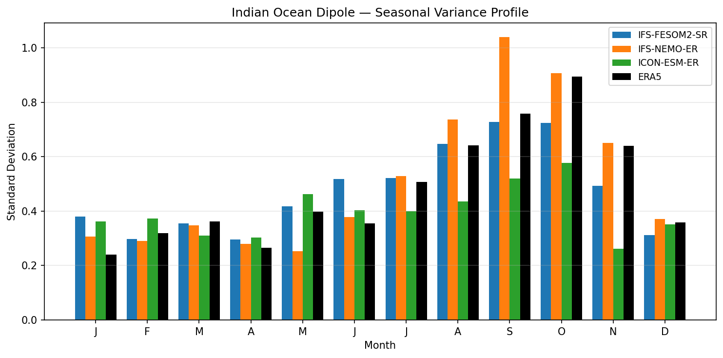
Indian Ocean Dipole — Seasonal Variance Profile
| Variables | tos |
|---|---|
| Models | IFS-FESOM2-SR, IFS-NEMO-ER, ICON-ESM-ER |
| Reference Dataset | ESA_CCI |
| Units | K |
| Period | 1980–2014 |
| IFS-FESOM2-SR | Peak Month: 9.00 · Peak Std: 0.73 · Annual Std: 0.50 |
| IFS-NEMO-ER | Peak Month: 9.00 · Peak Std: 1.04 · Annual Std: 0.57 |
| ICON-ESM-ER | Peak Month: 10.00 · Peak Std: 0.58 · Annual Std: 0.41 |
Summary high
This figure evaluates the seasonal variance of the Indian Ocean Dipole (IOD) index, revealing that IFS-FESOM2-SR best captures the observed seasonal cycle, whereas IFS-NEMO-ER overestimates and ICON-ESM-ER underestimates peak variability.
Key Findings
- ERA5 observations display the characteristic phase-locking of IOD variability, with a distinct peak in October (~0.9 K) and elevated variance throughout the boreal autumn (SON).
- IFS-NEMO-ER overestimates IOD variability, showing an overly intense peak in September (>1.0 K) that precedes the observed maximum.
- ICON-ESM-ER significantly underestimates IOD amplitude, with a peak standard deviation of only ~0.58 K in October, failing to reproduce the magnitude of the observed autumn intensification.
- IFS-FESOM2-SR provides the most accurate simulation of the seasonal cycle shape, though it slightly underestimates the peak magnitude (~0.73 K) compared to ERA5.
Spatial Patterns
All models reproduce the fundamental seasonality of the IOD, with variance minima in boreal spring (March-April) and maxima in boreal autumn (September-November).
Model Agreement
IFS-FESOM2-SR shows the highest agreement with observations regarding timing and cycle shape. IFS-NEMO-ER and ICON-ESM-ER diverge significantly in amplitude, bracketing the observations (one too strong, one too weak).
Physical Interpretation
The IOD is phase-locked to the boreal autumn due to seasonal changes in the thermocline and surface winds that maximize Bjerknes feedback efficiency. The excessive variability in IFS-NEMO-ER suggests overly sensitive air-sea coupling or a mean-state bias (e.g., excessively shallow eastern thermocline) that amplifies these feedbacks. Conversely, the damped variability in ICON-ESM-ER implies weak coupling or deep thermocline biases that inhibit the growth of SST anomalies.
Caveats
- Legend indicates ERA5 as the observational reference, while metadata lists ESA_CCI; though likely consistent, minor differences in SST products can exist.
- Analysis focuses on the dipole mode index variance and does not diagnose the specific spatial structural biases contributing to the index values.
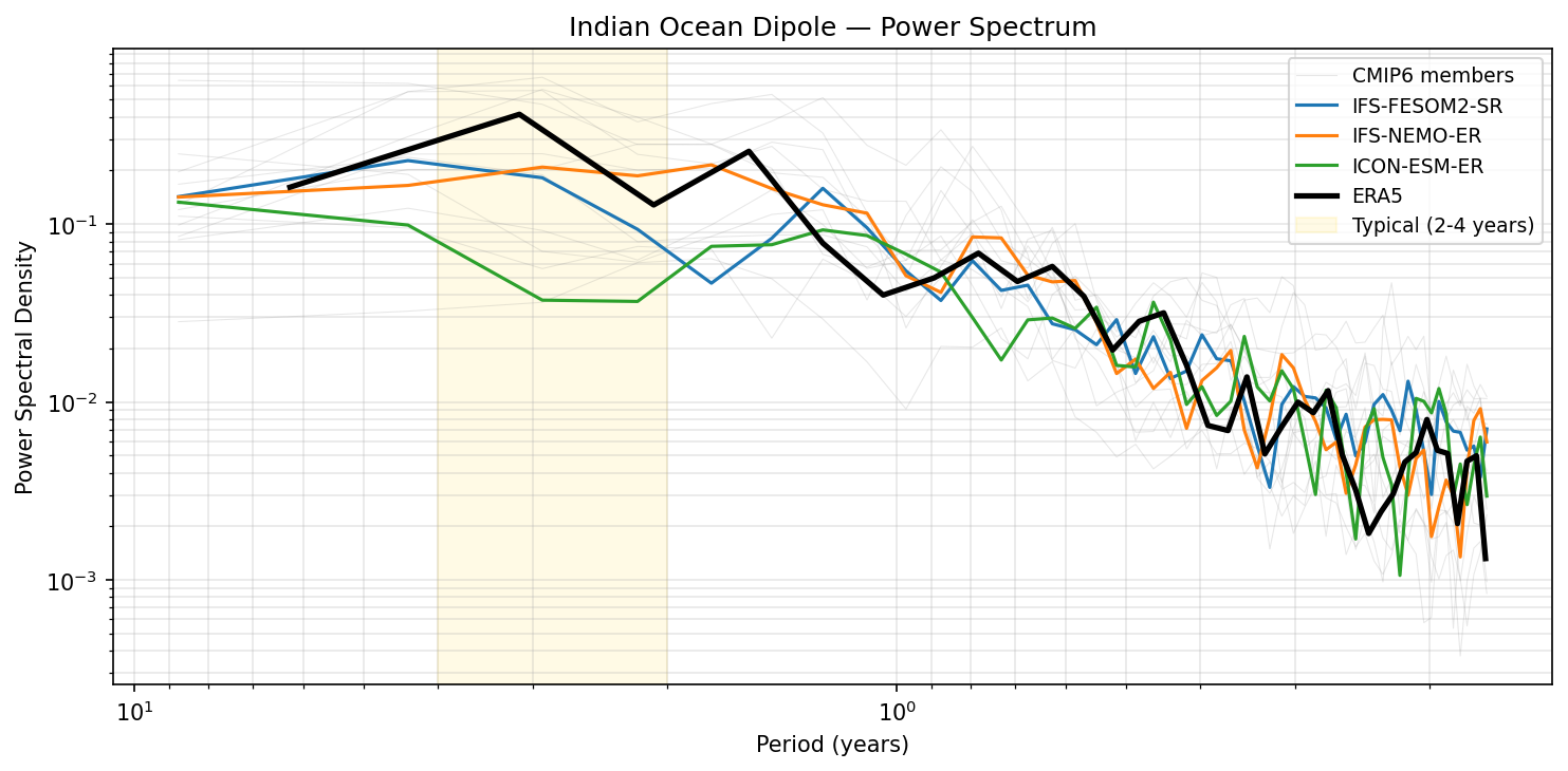
Indian Ocean Dipole — Power Spectrum
| Variables | tos |
|---|---|
| Models | IFS-FESOM2-SR, IFS-NEMO-ER, ICON-ESM-ER |
| Reference Dataset | ESA_CCI |
| Units | K |
| Period | 1980–2014 |
Summary high
This power spectrum analysis of the Indian Ocean Dipole (IOD) index reveals significant differences in how the evaluated models capture interannual variability, with IFS-NEMO-ER performing best while ICON-ESM-ER substantially underestimates variability.
Key Findings
- IFS-NEMO-ER most closely reproduces the observed (ERA5) spectral shape and power in the typical 2-4 year IOD band, though it slightly underestimates the peak magnitude.
- IFS-FESOM2-SR captures the general spectral decay but consistently underestimates the power spectral density in the critical 2-4 year range compared to ERA5 and IFS-NEMO-ER.
- ICON-ESM-ER fails to generate significant interannual variability, showing a flat spectrum with much lower power than observations and other models across the 2-10 year periods.
- ERA5 observations show a distinct peak in variability around 3-4 years, which is well-supported by the CMIP6 ensemble spread, whereas ICON-ESM-ER falls at the very bottom of or below the CMIP6 range.
Spatial Patterns
N/A (Frequency domain analysis). The dominant spectral feature in observations is the energy concentration in the 2-4 year band, indicative of the quasi-periodic nature of the IOD.
Model Agreement
There is notable divergence among the high-resolution models. IFS-NEMO-ER shows good agreement with ERA5, while IFS-FESOM2-SR is weaker, and ICON-ESM-ER shows poor agreement. All models tend to follow the high-frequency (sub-annual) decay of the observations reasonably well.
Physical Interpretation
The IOD relies on Bjerknes feedbacks involving wind-thermocline-SST interactions in the tropical Indian Ocean. The strong performance of IFS-NEMO-ER suggests its ocean mean state (e.g., thermocline depth) and coupling allow these feedbacks to operate effectively. Conversely, the dampened variability in ICON-ESM-ER and to a lesser extent IFS-FESOM2-SR (which shares the same atmosphere as IFS-NEMO) suggests potential biases in the ocean mean state or mixing processes that suppress the development of SST anomalies.
Caveats
- The analysis period (1980–2014) is relatively short for robust spectral density estimation of multi-year modes, though sufficient to distinguish gross differences.
- Discrepancies in observation labeling (Legend: ERA5 vs Metadata: ESA_CCI) suggest ERA5 reanalysis SSTs were used, which are observational estimates.
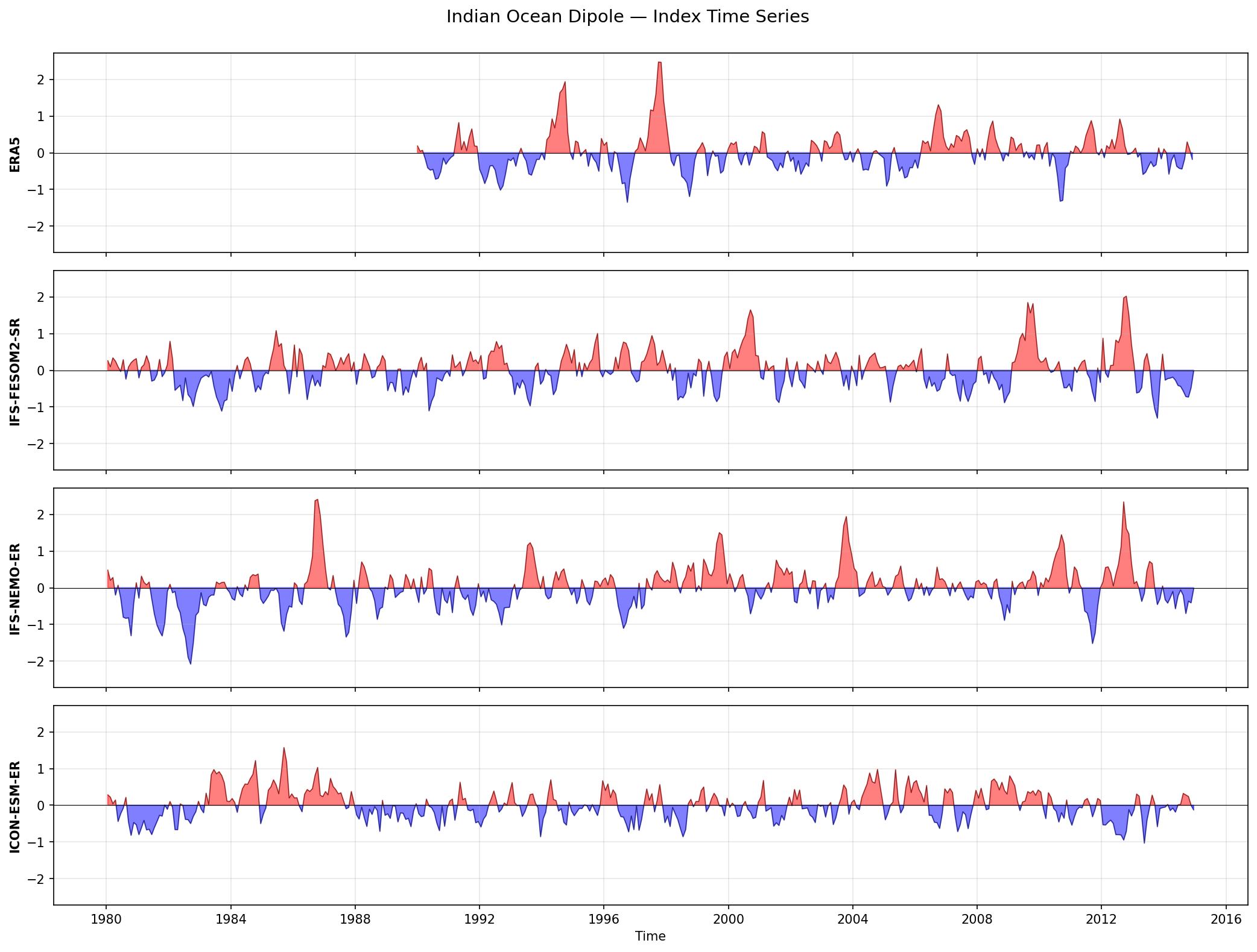
Indian Ocean Dipole — Index Time Series
| Variables | tos |
|---|---|
| Models | IFS-FESOM2-SR, IFS-NEMO-ER, ICON-ESM-ER |
| Reference Dataset | ESA_CCI |
| Units | K |
| Period | 1980–2014 |
| IFS-FESOM2-SR | Std: 0.50 · Mean: 0.00 |
| IFS-NEMO-ER | Std: 0.57 · Mean: 0.00 |
| ICON-ESM-ER | Std: 0.41 · Mean: -0.00 |
Summary high
This figure compares the time series of the Indian Ocean Dipole (IOD) index from 1980–2014 across three coupled climate models (IFS-FESOM2-SR, IFS-NEMO-ER, ICON-ESM-ER) against ERA5 observations. The models are free-running, so the analysis focuses on the statistical properties (amplitude and frequency) of variability rather than phase synchronization.
Key Findings
- IFS-NEMO-ER exhibits the highest variability (std ~0.57), producing strong positive IOD events with index values exceeding 2.0, comparable to the extreme 1997 event seen in observations.
- ICON-ESM-ER significantly underestimates IOD variability (std ~0.41), with index peaks rarely exceeding 1.0 and a visually dampened character compared to the other models and observations.
- IFS-FESOM2-SR shows moderate variability (std ~0.50), capturing the irregular periodicity of the IOD but generating fewer extreme amplitude events than IFS-NEMO-ER.
- ERA5 observations show characteristic strong positive events (e.g., 1997, 2006) and negative events (e.g., 1998, 2010), serving as a benchmark for potential event magnitude.
Spatial Patterns
N/A (Time series analysis). Temporally, all models reproduce the irregular interannual oscillation characteristic of the IOD (typically 2-5 year recurrence), though ICON-ESM-ER shows slightly more persistent, less 'spiky' behavior.
Model Agreement
There is significant divergence in the amplitude of simulated variability. IFS-NEMO-ER is the most energetic, likely closest to the observed distribution of extremes, while ICON-ESM-ER is the least energetic. IFS-FESOM2-SR lies in between. As these are uncoupled historical runs, event timing does not match observations.
Physical Interpretation
The differences in variability likely stem from the ocean components (NEMO vs. FESOM vs. ICON-O) and their coupling with the atmosphere. The IOD relies on Bjerknes feedbacks and thermocline dynamics in the equatorial Indian Ocean. The dampened variability in ICON-ESM-ER suggests potential biases in the mean state (e.g., a too-deep thermocline or weak zonal wind response) that suppress the growth of anomalies. Conversely, IFS-NEMO-ER appears to maintain a stratification or coupling strength that supports robust mode growth.
Caveats
- The ERA5 observational time series is truncated, showing data only from ~1990 onwards, hindering comparison for the 1980-1990 period.
- Since simulations are free-running, no correspondence in the timing of specific years (like the 1997 El Niño/IOD) is expected or observed.
North Atlantic Oscillation — Spatial Pattern
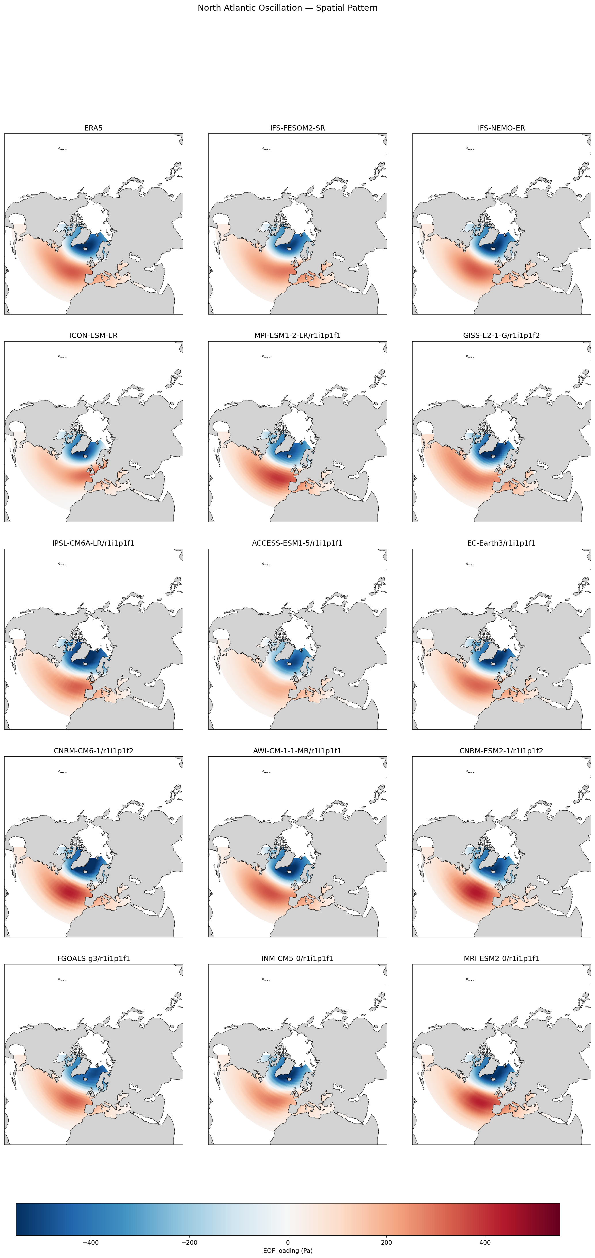
| Variables | psl |
|---|---|
| Models | IFS-FESOM2-SR, IFS-NEMO-ER, ICON-ESM-ER |
| Reference Dataset | ERA5 |
| Units | Pa |
| Period | 1980–2014 |
| IFS-FESOM2-SR | Variance Explained: 0.33 |
| IFS-NEMO-ER | Variance Explained: 0.35 |
| ICON-ESM-ER | Variance Explained: 0.27 |
| ERA5 | Variance Explained: 0.35 |
Summary high
This figure evaluates the spatial structure and explained variance of the North Atlantic Oscillation (NAO) in three high-resolution coupled models (IFS-FESOM2-SR, IFS-NEMO-ER, ICON-ESM-ER) and a CMIP6 ensemble compared to ERA5 reanalysis.
Key Findings
- All three high-resolution EERIE models successfully reproduce the classic NAO dipole pattern, with a negative node over the Icelandic/Greenland region and a positive node extending from the Azores to Europe.
- IFS-NEMO-ER shows remarkable agreement with ERA5 in terms of explained variance (35.3% vs 34.7% in ERA5) and spatial fidelity.
- ICON-ESM-ER captures the spatial pattern well but underestimates the explained variance (27.1%), indicating the NAO mode dominates the total variability less than in observations.
- The high-resolution models compare favorably to the CMIP6 ensemble, which generally captures the pattern but shows greater inter-model diversity in the amplitude and precise location of the centers of action (e.g., MRI-ESM2-0 showing a particularly intense positive pole).
Spatial Patterns
The dominant pattern is a north-south pressure dipole over the North Atlantic. The negative pole (Icelandic Low) is centered between Greenland and Iceland, while the positive pole (Azores High) spans the subtropical Atlantic towards the Iberian Peninsula. The EOF loading magnitudes are typically ±400 Pa (4 hPa) per standard deviation.
Model Agreement
There is high agreement on the gross spatial structure across all models shown. IFS-NEMO-ER and IFS-FESOM2-SR are particularly close to ERA5 in both pattern shape and variance explained (32-35%). ICON-ESM-ER is an outlier among the high-res group regarding variance explained (27%), though its spatial pattern remains consistent with the others. Some CMIP6 models (e.g., ACCESS-ESM1-5) appear visually weaker or have slightly shifted centers compared to the IFS/ERA5 baseline.
Physical Interpretation
The NAO represents the leading mode of atmospheric mass variability in the North Atlantic sector, driven by the internal dynamics of the atmospheric jet stream and storm tracks. The successful replication of this pattern implies that the models correctly simulate the mean position and variability of the Atlantic jet and the associated eddy-mean flow interactions. The correct variance explained in IFS models suggests realistic storm track activity levels.
Caveats
- Analysis is based on the first EOF only; higher-order modes are not evaluated.
- The specific time periods for CMIP6 models vs the EERIE simulations (1980-2014) should be confirmed to ensure strict comparability, though broad climatological features are robust.
North Atlantic Oscillation — Seasonal Variance Profile
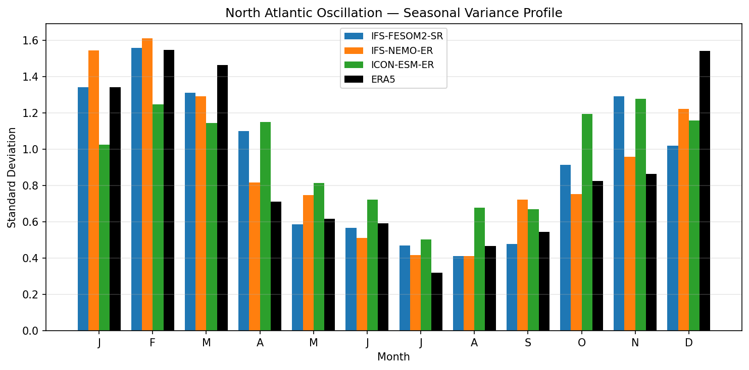
| Variables | psl |
|---|---|
| Models | IFS-FESOM2-SR, IFS-NEMO-ER, ICON-ESM-ER |
| Reference Dataset | ERA5 |
| Units | Pa |
| Period | 1980–2014 |
| IFS-FESOM2-SR | Peak Month: 2.00 · Peak Std: 1.56 · Annual Std: 1.00 |
| IFS-NEMO-ER | Peak Month: 2.00 · Peak Std: 1.61 · Annual Std: 1.00 |
| ICON-ESM-ER | Peak Month: 11.00 · Peak Std: 1.28 · Annual Std: 1.00 |
Summary high
The figure illustrates the seasonal cycle of North Atlantic Oscillation (NAO) variability, comparing the monthly standard deviation of the NAO index in three high-resolution models against ERA5 reanalysis. While IFS models generally reproduce the characteristic winter variability maximum, ICON-ESM-ER exhibits a flattened seasonal cycle with a shifted peak and excessive variability during transition seasons.
Key Findings
- ERA5 displays a robust seasonal cycle with variability peaking in December and February (~1.55 standard deviation) and minimizing in July (~0.3).
- IFS-FESOM2-SR and IFS-NEMO-ER accurately capture the February peak magnitude, but all three models underestimate the December variability peak (models ~1.0–1.2 vs ERA5 ~1.55).
- ICON-ESM-ER fails to capture the winter dominance, with its variability peaking anomalously in November (~1.28) rather than DJF, and generally underestimates true winter variability.
- Significant model spread exists in April: IFS-FESOM2-SR and ICON-ESM-ER overestimate variability (~1.1–1.15 vs ERA5 ~0.7), while IFS-NEMO-ER tracks the observational decline closely.
Spatial Patterns
N/A (Temporal profile). The observations show a clear sinusoidal seasonal dependence rooted in the boreal winter intensification of the Atlantic jet stream.
Model Agreement
The two IFS-based models (FESOM and NEMO) show better agreement with the observed winter peak structure (Jan-Feb) than ICON. However, all models struggle to reproduce the high variability observed in December. ICON is an outlier with high biases in Oct-Nov and Apr-May.
Physical Interpretation
The NAO reflects variability in the North Atlantic eddy-driven jet. The collective underestimation of December variance suggests models may delay the onset of the most vigorous winter storm track regime or miss early-winter stratosphere-troposphere coupling signals. The spurious April variability peaks in IFS-FESOM2-SR and ICON-ESM-ER suggest an inability to transition promptly from winter-like baroclinic instability to the more stable spring circulation.
Caveats
- The analysis focuses on variance amplitude, not the spatial fidelity of the NAO pattern itself.
- Differences in ocean coupling (FESOM vs NEMO) in the IFS models appear to influence the spring transition (April) significantly.
North Atlantic Oscillation — Power Spectrum
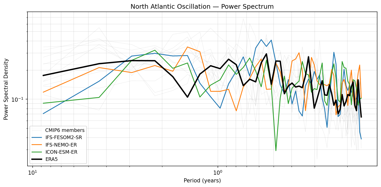
| Variables | psl |
|---|---|
| Models | IFS-FESOM2-SR, IFS-NEMO-ER, ICON-ESM-ER |
| Reference Dataset | ERA5 |
| Units | Pa |
| Period | 1980–2014 |
Summary medium
The power spectra of the North Atlantic Oscillation (NAO) for the evaluated high-resolution models generally reproduce the observed broadband, quasi-red noise character of ERA5, falling within the wider CMIP6 ensemble spread.
Key Findings
- IFS-NEMO-ER and IFS-FESOM2-SR exhibit elevated power spectral density in the interannual band (2–5 year periods) compared to ERA5, suggesting slightly excessive persistence or variability at these timescales.
- ICON-ESM-ER shows lower power at decadal timescales (periods > 8 years) compared to ERA5 and the IFS models.
- ICON-ESM-ER displays a distinct, anomalous drop in spectral density at sub-annual periods (approx. 0.7–0.8 years) not seen in observations or other models.
- All three high-resolution models generally fall within the envelope of the CMIP6 members, indicating their NAO temporal variability is comparable to standard-resolution coupled models.
Spatial Patterns
N/A (Frequency domain analysis of a scalar index).
Model Agreement
The two IFS-based models (NEMO and FESOM2) show strong agreement with each other, particularly in the 2–5 year excess power band, implying this is an atmospheric model characteristic. ICON-ESM-ER diverges with lower low-frequency energy.
Physical Interpretation
The NAO is primarily an internal atmospheric mode with a spectrum close to white or red noise. The excess interannual power in IFS models may indicate overly strong coupling to lower-frequency oceanic drivers (e.g., SST anomalies or ENSO teleconnections) or intrinsic atmospheric persistence. The reduced low-frequency power in ICON suggests a lack of long-term memory in its North Atlantic jet dynamics.
Caveats
- The 35-year analysis period (1980–2014) is short for robustly estimating spectral density at decadal periods (left side of plot).
- Spectra are naturally noisy; differences in peaks may partly result from internal variability sampling rather than systematic model errors.
North Atlantic Oscillation — Index Time Series
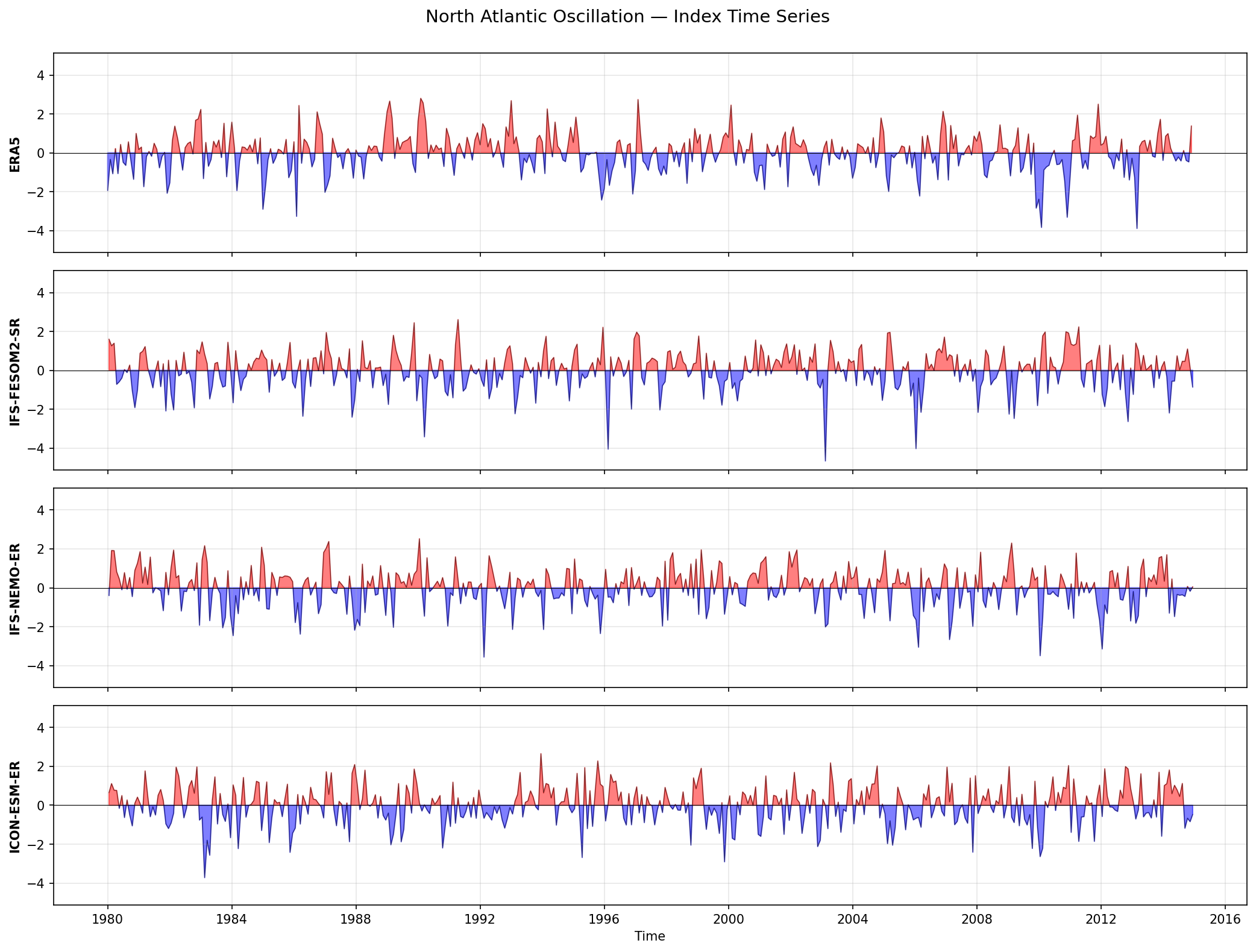
| Variables | psl |
|---|---|
| Models | IFS-FESOM2-SR, IFS-NEMO-ER, ICON-ESM-ER |
| Reference Dataset | ERA5 |
| Units | Pa |
| Period | 1980–2014 |
| IFS-FESOM2-SR | Std: 1.00 · Mean: -0.00 |
| IFS-NEMO-ER | Std: 1.00 · Mean: 0.00 |
| ICON-ESM-ER | Std: 1.00 · Mean: 0.00 |
Summary high
This diagnostic displays the standardized monthly North Atlantic Oscillation (NAO) index time series for ERA5 reanalysis and three high-resolution coupled models (IFS-FESOM2-SR, IFS-NEMO-ER, ICON-ESM-ER) over the period 1980–2014.
Key Findings
- All three models reproduce the statistical range and variability of the observed NAO, with index values fluctuating typically between ±3, consistent with ERA5.
- The models exhibit realistic frequency characteristics, showing a mix of high-frequency monthly noise and interannual variability without distinct pathological locking into positive or negative phases.
- Extreme NAO events (magnitude > 3) are simulated in all models, with IFS-FESOM2-SR producing a notable negative excursion (<-4) similar in magnitude to the extreme 2009/2010 winter event seen in ERA5.
- Metadata statistics confirm that all models have a standard deviation of ~1.0, indicating successful identification and normalization of the NAO mode relative to each model's internal climatology.
Spatial Patterns
While strictly a temporal view, the time series demonstrate that the models capture the episodic nature of the NAO. The distribution of positive (red) and negative (blue) anomalies appears visually balanced in all simulations, similar to the reanalysis.
Model Agreement
The models show high agreement with observations regarding the amplitude and statistical character of the variability. As these are free-running coupled simulations, the specific timing of phases does not (and should not be expected to) correlate with the historical ERA5 timeline.
Physical Interpretation
The realistic amplitude of the index implies that the models correctly simulate the magnitude of the pressure dipole between the Icelandic Low and Azores High, as well as the associated latitudinal shifts of the North Atlantic eddy-driven jet. The presence of reasonable interannual variability suggests the models capture the internal atmospheric dynamics and potential ocean-atmosphere coupling mechanisms that sustain the NAO.
Caveats
- The figure evaluates the temporal projection of the mode but does not assess the spatial fidelity of the teleconnection pattern (e.g., the exact location of the centers of action).
- Direct temporal correlation with ERA5 is not a valid performance metric for these uninitialized simulations.
Pacific Decadal Oscillation — Spatial Pattern
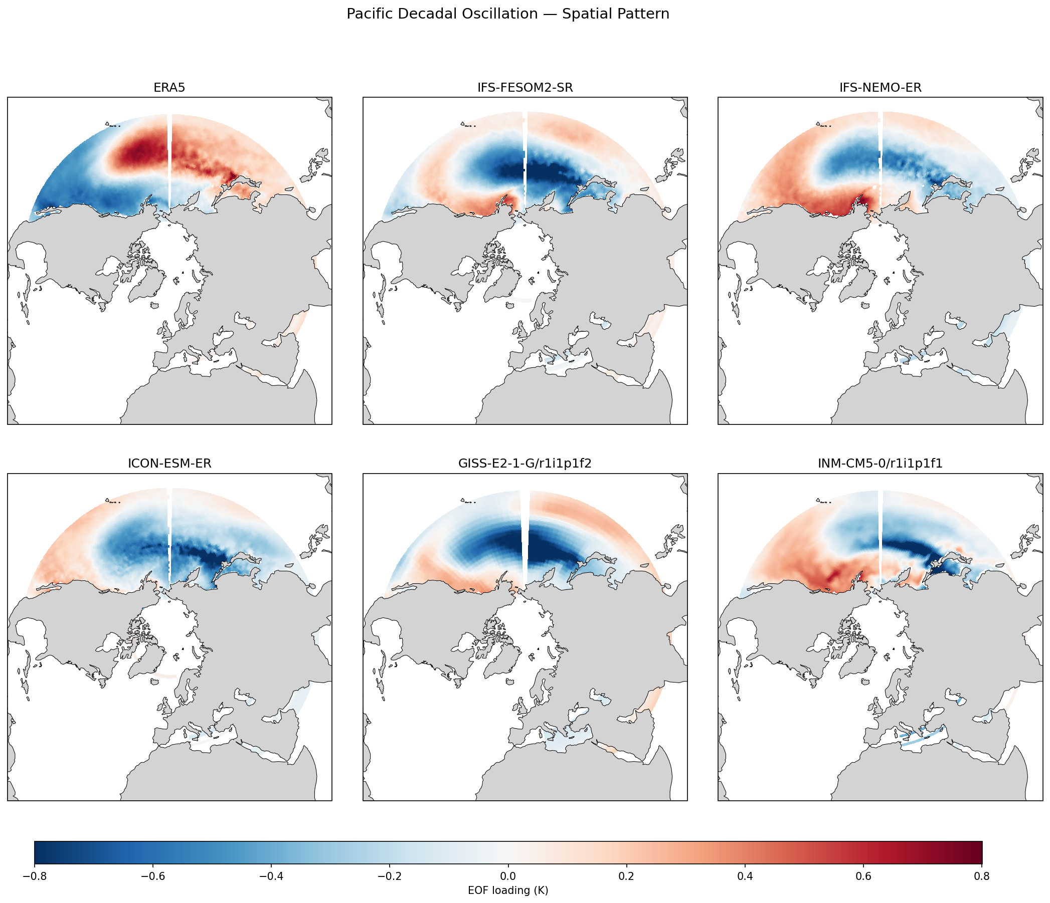
| Variables | tos |
|---|---|
| Models | IFS-FESOM2-SR, IFS-NEMO-ER, ICON-ESM-ER |
| Reference Dataset | ESA_CCI |
| Units | K |
| Period | 1980–2014 |
| IFS-FESOM2-SR | Variance Explained: 0.14 |
| IFS-NEMO-ER | Variance Explained: 0.12 |
| ICON-ESM-ER | Variance Explained: 0.13 |
| ERA5 | Variance Explained: 0.19 |
Summary high
This figure evaluates the spatial pattern of the Pacific Decadal Oscillation (PDO) based on the first EOF of SST anomalies (1980–2014). While all evaluated high-resolution models capture the primary action center in the central North Pacific, IFS-NEMO-ER demonstrates superior skill in reproducing the canonical 'horseshoe' pattern along the North American coast compared to IFS-FESOM2-SR and ICON-ESM-ER.
Key Findings
- IFS-NEMO-ER shows the most realistic spatial structure, correctly capturing the magnitude and extent of the coastal anomaly (Alaska to California) that opposes the central Pacific core.
- IFS-FESOM2-SR and ICON-ESM-ER correctly simulate the central North Pacific anomaly but fail to reproduce the connected eastern boundary signal, resulting in a disconnected or weak coastal 'horseshoe'.
- All models underestimate the variance explained by the PDO mode (ranging from 12.1% to 13.6%) compared to ERA5 (19.3%), suggesting the modeled PDO is less dominant relative to other variability than in observations.
Spatial Patterns
ERA5 shows a distinct dipole structure: a strong anomaly in the Kuroshio-Oyashio Extension (KOE) region and an opposing anomaly wrapping along the North American west coast. IFS-NEMO-ER reproduces this dipole well (albeit with flipped EOF sign). In contrast, IFS-FESOM2-SR and ICON-ESM-ER exhibit a zonally elongated central anomaly that dominates the EOF, with the eastern coastal branch appearing washed out or absent.
Model Agreement
IFS-NEMO-ER agrees best with observations spatially. IFS-FESOM2-SR and ICON-ESM-ER cluster together with similar structural deficiencies in the eastern Pacific. The CMIP6 models (GISS, INM) included for context show coarser patterns that lack the sharp frontal definition seen in the high-resolution simulations.
Physical Interpretation
The PDO is driven by the integration of atmospheric noise (Aleutian Low) and ENSO teleconnections. The failure of FESOM and ICON to capture the coastal branch suggests potential biases in the atmospheric bridge (PNA pattern) reaching the coast or deficiencies in resolving coastal upwelling dynamics in the California Current system. The sharper KOE front in the high-res models reflects the role of ocean resolution in maintaining western boundary current gradients.
Caveats
- The sign of EOF patterns is arbitrary; the fact that models show the opposite polarity to ERA5 is a mathematical convention, not a physical bias.
- The 35-year analysis period is short for characterizing decadal variability, capturing only limited phase transitions.
Pacific Decadal Oscillation — Seasonal Variance Profile
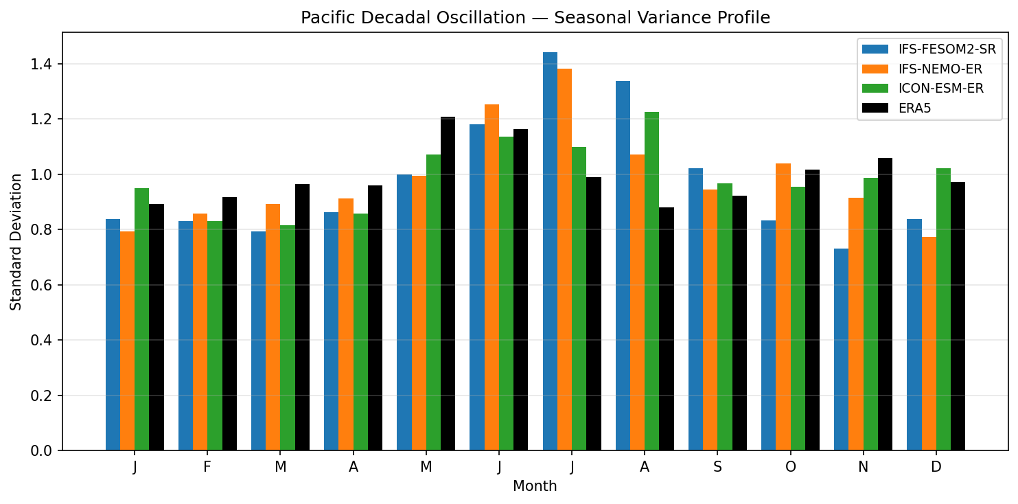
| Variables | tos |
|---|---|
| Models | IFS-FESOM2-SR, IFS-NEMO-ER, ICON-ESM-ER |
| Reference Dataset | ESA_CCI |
| Units | K |
| Period | 1980–2014 |
| IFS-FESOM2-SR | Peak Month: 7.00 · Peak Std: 1.44 · Annual Std: 1.00 |
| IFS-NEMO-ER | Peak Month: 7.00 · Peak Std: 1.38 · Annual Std: 1.00 |
| ICON-ESM-ER | Peak Month: 8.00 · Peak Std: 1.22 · Annual Std: 1.00 |
Summary high
This figure evaluates the seasonal cycle of Pacific Decadal Oscillation (PDO) variability, revealing that all coupled models exhibit a delayed and exaggerated peak in variance compared to ERA5.
Key Findings
- ERA5 observations show peak PDO variability in late spring (May-June, ~1.2 SD), whereas the models simulate peak variability in high summer (July for IFS models, August for ICON).
- IFS-FESOM2-SR and IFS-NEMO-ER substantially overestimate PDO variance in July (reaching ~1.4 SD compared to ERA5's ~1.0 SD), indicating excessive sensitivity during the summer months.
- ICON-ESM-ER displays a delayed peak (August) like the IFS models but maintains variance magnitudes closer to observations in winter months compared to the IFS variants.
Spatial Patterns
N/A (Temporal profile shown). The dominant temporal feature is the shift from a spring maximum in observations to a summer maximum in simulations.
Model Agreement
The two IFS-based models (NEMO and FESOM) show high agreement in their seasonal profile, sharing the distinct July spike. ICON-ESM-ER is distinct with a flatter profile and an August peak, suggesting the atmospheric component (IFS vs ICON) or coupling implementation influences the timing.
Physical Interpretation
The PDO reflects the integration of atmospheric noise by the ocean mixed layer. The excessive summer variance in models suggests the simulated mixed layer depth (MLD) in the North Pacific may be too shallow in summer (reducing thermal inertia) or that surface heat flux damping is too weak. The phase delay in peak variability implies errors in the seasonal cycle of the Aleutian Low forcing or the timing of MLD shoaling.
Caveats
- The PDO index assumes the underlying spatial EOF patterns are consistent between models and observations; spatial biases in the North Pacific mode could project onto this variance metric.
- The use of 'ERA5' in the legend vs 'ESA_CCI' in metadata suggests reanalysis SSTs, which are generally reliable but depend on assimilation quality.
Pacific Decadal Oscillation — Power Spectrum
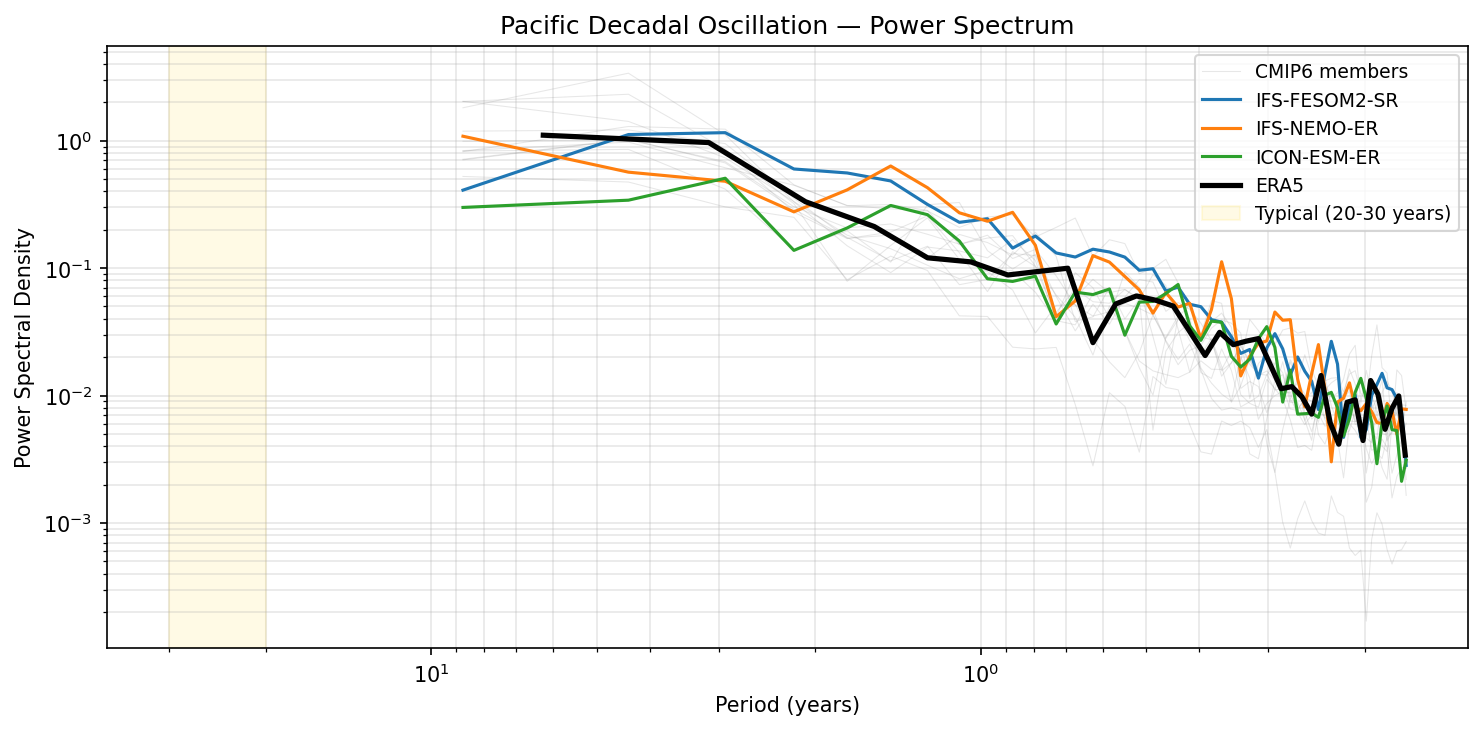
| Variables | tos |
|---|---|
| Models | IFS-FESOM2-SR, IFS-NEMO-ER, ICON-ESM-ER |
| Reference Dataset | ESA_CCI |
| Units | K |
| Period | 1980–2014 |
Summary medium
This power spectrum analysis of the Pacific Decadal Oscillation (PDO) index (1980–2014) evaluates whether models capture the intensity of variability across different timescales. The IFS-based models closely match the observed (ERA5) spectral power, whereas ICON-ESM-ER systematically underestimates variability across interannual to decadal frequencies.
Key Findings
- IFS-FESOM2-SR and IFS-NEMO-ER reproduce the observed spectral power density well across the resolved periods (1 to ~15 years), tracking the ERA5 reference closely.
- ICON-ESM-ER consistently exhibits weaker variability than observations and the other high-resolution models, falling near the lower bound of the CMIP6 ensemble spread.
- All models capture the general 'red noise' characteristics of the spectrum (power increasing with period) and the ENSO-related variability peaks in the 3–7 year band.
- The analysis period (35 years) is insufficient to resolve the canonical 20–30 year PDO timescale (highlighted by the yellow band), meaning the diagnostic primarily assesses the interannual to decadal projection of the PDO.
Spatial Patterns
While this is a frequency-domain plot, the spectrum reveals structure in the time domain: a dominance of low-frequency variability (red noise) and distinct enhancements in the 3–7 year ENSO band, which projects strongly onto the PDO index in all datasets.
Model Agreement
There is strong agreement between IFS-FESOM2-SR, IFS-NEMO-ER, and ERA5. In contrast, ICON-ESM-ER diverges significantly with dampened power. All high-resolution models fall within the wide spread of the standard-resolution CMIP6 ensemble.
Physical Interpretation
The PDO is largely an integration of atmospheric noise and ENSO teleconnections. The realistic spectra in IFS models suggest they capture both the local North Pacific atmospheric forcing and the remote ENSO bridging mechanism effectively. The damped variability in ICON-ESM-ER suggests either a weak ENSO amplitude in this model or excessive damping of SST anomalies in the North Pacific mixed layer.
Caveats
- The 1980–2014 analysis window is too short to statistically resolve the multidecadal (20–30 year) component of the PDO, limiting the evaluation to higher-frequency components.
- Spectral estimates at the longest resolved periods (>10 years) are subject to high uncertainty due to the limited number of realizations in the short record.
Pacific Decadal Oscillation — Index Time Series
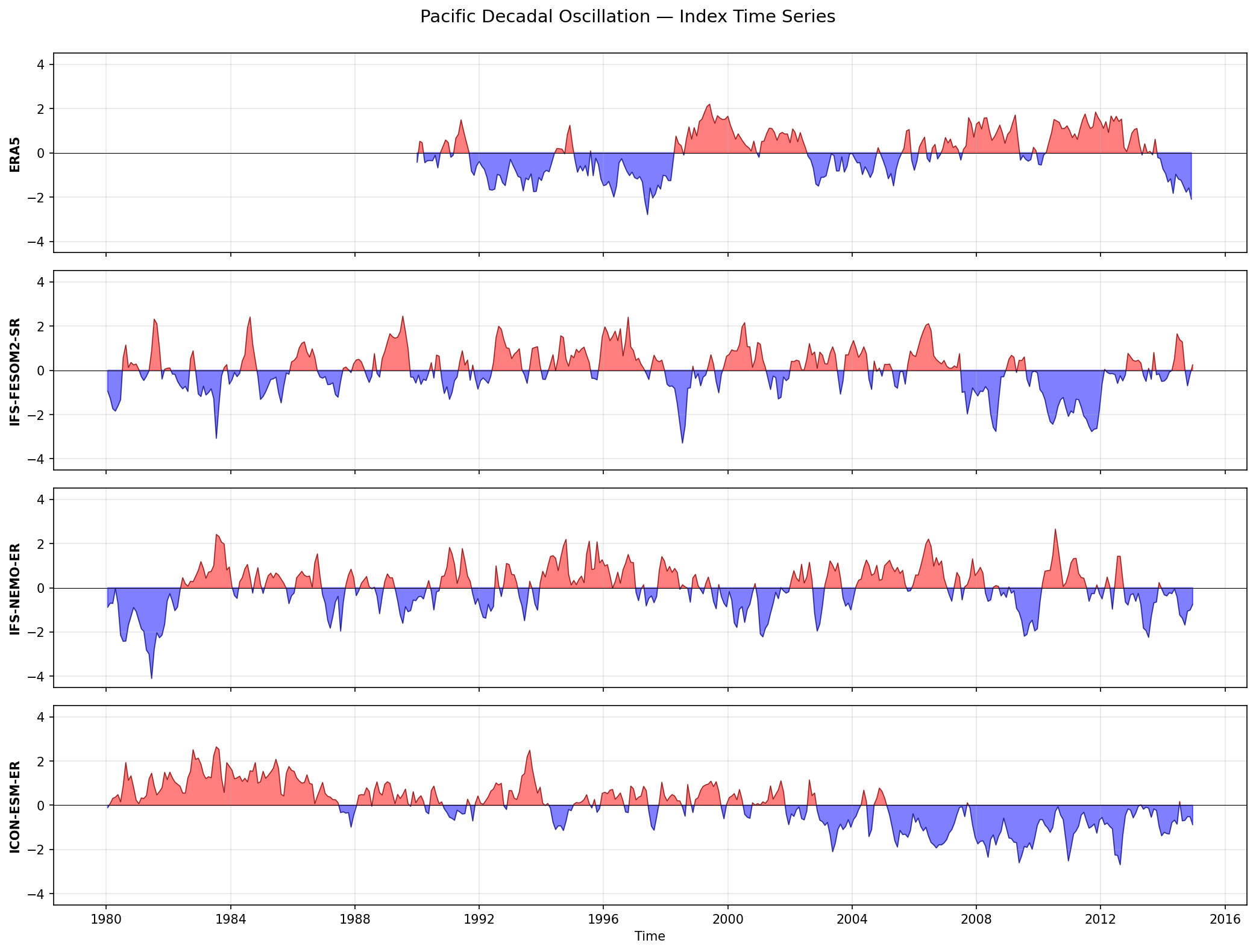
| Variables | tos |
|---|---|
| Models | IFS-FESOM2-SR, IFS-NEMO-ER, ICON-ESM-ER |
| Reference Dataset | ESA_CCI |
| Units | K |
| Period | 1980–2014 |
| IFS-FESOM2-SR | Std: 1.00 · Mean: -0.00 |
| IFS-NEMO-ER | Std: 1.00 · Mean: -0.00 |
| ICON-ESM-ER | Std: 1.00 · Mean: 0.00 |
Summary medium
This figure displays the time series of the Pacific Decadal Oscillation (PDO) index from 1980 to 2014 for ERA5 reanalysis (labelled, though data appears truncated) and three high-resolution coupled climate models (IFS-FESOM2-SR, IFS-NEMO-ER, ICON-ESM-ER). The plot highlights significant differences in the dominant timescales of variability between the ICON and IFS model families.
Key Findings
- ICON-ESM-ER exhibits distinct multi-decadal persistence, maintaining a positive phase from ~1980–1994 and a negative phase from ~2003–2014, contrasting with the more frequent phase flipping seen in other models.
- IFS-FESOM2-SR and IFS-NEMO-ER show higher-frequency variability with phase transitions often occurring every 3–5 years, suggesting a stronger influence of interannual (ENSO-like) variability rather than sustained decadal regimes.
- The ERA5 observational panel appears to be missing data prior to ~1990, limiting the visual comparison for the first decade of the analysis period.
- IFS-NEMO-ER exhibits the most extreme excursion, with a negative spike reaching -4 standard deviations around 1981.
Spatial Patterns
Not applicable (time series only), though the temporal patterns indicate that ICON-ESM-ER produces longer-duration 'regimes' (10+ years) compared to the shorter duration anomalies in the IFS-based models.
Model Agreement
As these are free-running coupled simulations, phase agreement with observations or between models is not expected (internal variability). However, there is a divergence in the *character* of variability: ICON supports lower-frequency modes, while IFS models are dominated by higher-frequency fluctuations.
Physical Interpretation
The PDO is often conceptualised as the 'reddening' of ENSO variability by the North Pacific Ocean's thermal inertia. The persistent regimes in ICON-ESM-ER suggest either a lower-frequency ENSO driver, stronger ocean memory mechanisms, or weaker damping in the North Pacific compared to the IFS models. The IFS models' behavior implies a tighter coupling to interannual atmospheric forcing (SST tracking the atmosphere) rather than oceanic integration.
Caveats
- The analysis period (1980–2014) is very short for evaluating decadal variability; typically only 1–2 full cycles can be observed, limiting statistical robustness.
- The missing data in the ERA5 panel for the 1980s prevents a complete baseline comparison for regime duration.
- Standardised indices (std=1) mask differences in absolute SST anomaly variance.
Quasi-Biennial Oscillation — Spatial Pattern
| Variables | ua |
|---|---|
| Models | IFS-FESOM2-SR, IFS-NEMO-ER, ICON-ESM-ER |
| Reference Dataset | ERA5 |
| Units | m/s |
| Period | 1980–2014 |
Summary high
The provided figure is a placeholder indicating that no spatial pattern diagnostic was generated for the Quasi-Biennial Oscillation (QBO) within this specific teleconnection analysis suite.
Key Findings
- The figure contains no data or plotted fields.
- A text annotation states 'No spatial pattern for Quasi-Biennial Oscillation'.
- This diagnostic likely excludes QBO spatial maps because the mode is primarily defined by vertical propagation (time-height) rather than horizontal spatial covariance.
Spatial Patterns
No spatial patterns are displayed.
Model Agreement
Cannot be assessed as no model data is present.
Physical Interpretation
The QBO is characterized by alternating easterly and westerly wind regimes propagating downward in the tropical stratosphere. While it impacts global circulation, the mode itself is best visualized via vertical profiles or time-height sections of zonal wind (e.g., at the equator) rather than a static horizontal EOF or regression map commonly used for modes like the NAO or PNA.
Caveats
- The figure is entirely empty of data.
- Analysis of QBO performance requires looking at specific time-height or spectral diagnostics, not this placeholder.
Quasi-Biennial Oscillation — Seasonal Variance Profile
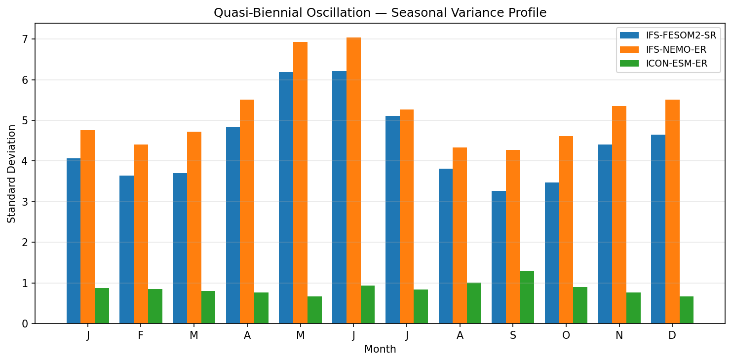
| Variables | ua |
|---|---|
| Models | IFS-FESOM2-SR, IFS-NEMO-ER, ICON-ESM-ER |
| Reference Dataset | ERA5 |
| Units | m/s |
| Period | 1980–2014 |
| IFS-FESOM2-SR | Peak Month: 6.00 · Peak Std: 6.22 · Annual Std: 4.55 |
| IFS-NEMO-ER | Peak Month: 6.00 · Peak Std: 7.04 · Annual Std: 5.30 |
| ICON-ESM-ER | Peak Month: 9.00 · Peak Std: 1.29 · Annual Std: 0.88 |
Summary high
This figure compares the seasonal variance profile of the Quasi-Biennial Oscillation (QBO) index across three models, revealing a fundamental dichotomy: IFS-based models reproduce a robust oscillation, while ICON-ESM-ER fails to generate a meaningful signal.
Key Findings
- ICON-ESM-ER shows negligible QBO variability with standard deviations consistently below 1.3 m/s, effectively indicating the absence of a QBO.
- IFS-NEMO-ER exhibits the highest variability, with a peak standard deviation of ~7.0 m/s in June.
- IFS-FESOM2-SR produces a robust signal similar in phase to IFS-NEMO-ER but with lower amplitude (peak ~6.2 m/s), consistently 0.5-1.0 m/s weaker than the eddy-rich IFS configuration.
Spatial Patterns
While the QBO is an interannual oscillation, the IFS models show a distinct seasonal modulation of its variance (temporal pattern), peaking in boreal late spring/summer (May-July) and reaching a minimum in autumn (September-October).
Model Agreement
There is strong disagreement between model families. The two IFS simulations agree on the existence and phasing of the variability, while ICON-ESM-ER diverges completely by lacking the phenomenon.
Physical Interpretation
The QBO relies on wave-mean flow interactions involving gravity, Kelvin, and Rossby-gravity waves. The absence of QBO in ICON-ESM-ER suggests insufficient vertical resolution in the stratosphere or inadequate non-orographic gravity wave drag parameterization. The higher variability in IFS-NEMO-ER compared to IFS-FESOM2-SR likely results from higher horizontal resolution resolving a greater flux of upward-propagating waves.
Caveats
- The observational reference (ERA5) mentioned in the metadata is not plotted, preventing verification of which model's amplitude is more realistic.
- Metadata refers to 'u10' (10m wind) which is incorrect for QBO (stratospheric); the analysis assumes the correct stratospheric zonal wind ('ua') was used.
Quasi-Biennial Oscillation — Power Spectrum
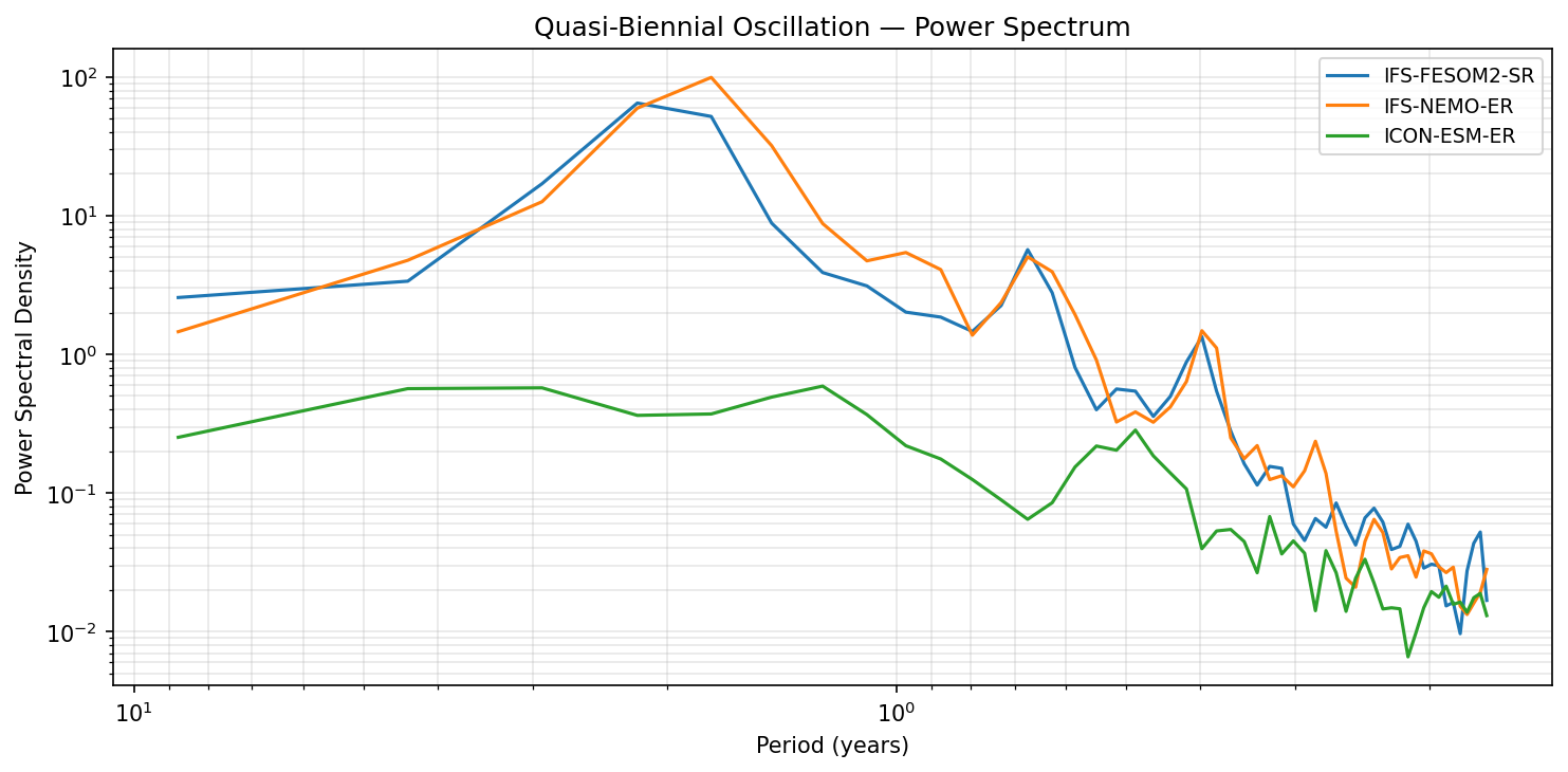
| Variables | ua |
|---|---|
| Models | IFS-FESOM2-SR, IFS-NEMO-ER, ICON-ESM-ER |
| Reference Dataset | ERA5 |
| Units | m/s |
| Period | 1980–2014 |
Summary high
This power spectrum analysis of the Quasi-Biennial Oscillation (QBO) reveals a stark contrast in model performance: the two IFS-based models reproduce a realistic QBO signal, while ICON-ESM-ER completely fails to generate the oscillation.
Key Findings
- IFS-NEMO-ER and IFS-FESOM2-SR exhibit a prominent spectral peak between 2 and 3 years, consistent with the observed ~28-month (2.33-year) QBO period.
- ICON-ESM-ER shows no spectral peak in the interannual range and has power spectral density values two orders of magnitude lower than the IFS models (peak < 1 vs ~100), indicating a complete absence of the QBO.
- IFS-NEMO-ER displays slightly higher power at the QBO peak compared to IFS-FESOM2-SR, but both share nearly identical spectral shapes, including secondary variability at sub-annual timescales.
Spatial Patterns
The primary feature is the dominant peak centered around ~2.3–2.5 years in the IFS models, typical of the QBO. Secondary spectral features appear in the sub-annual range (periods < 1 year), possibly related to the Semi-Annual Oscillation (SAO) or harmonics, which are visible in IFS but absent or buried in noise in ICON.
Model Agreement
There is high agreement between the two IFS configurations (IFS-FESOM2-SR and IFS-NEMO-ER), which differ primarily in ocean coupling, suggesting the QBO is robustly simulated by the atmospheric component. There is complete disagreement between the IFS family and ICON-ESM-ER.
Physical Interpretation
The QBO is driven by the interaction of upward-propagating waves (Kelvin, Rossby-gravity, and smaller-scale gravity waves) with the stratospheric mean flow. The success of the IFS models implies sufficient vertical resolution in the stratosphere and effective parameterization of non-orographic gravity wave drag. The failure of ICON-ESM-ER suggests it likely lacks the necessary vertical resolution or appropriate gravity wave tuning to spontaneously generate this stratospheric oscillation.
Caveats
- An observational reference line (e.g., ERA5) is listed in the metadata but is absent from the plot; assessment relies on the well-known ~28-month periodicity of the QBO.
- The analysis period (1980–2014) captures only about 15 QBO cycles, so small differences in peak magnitude between IFS runs may be due to internal variability.
Quasi-Biennial Oscillation — Index Time Series
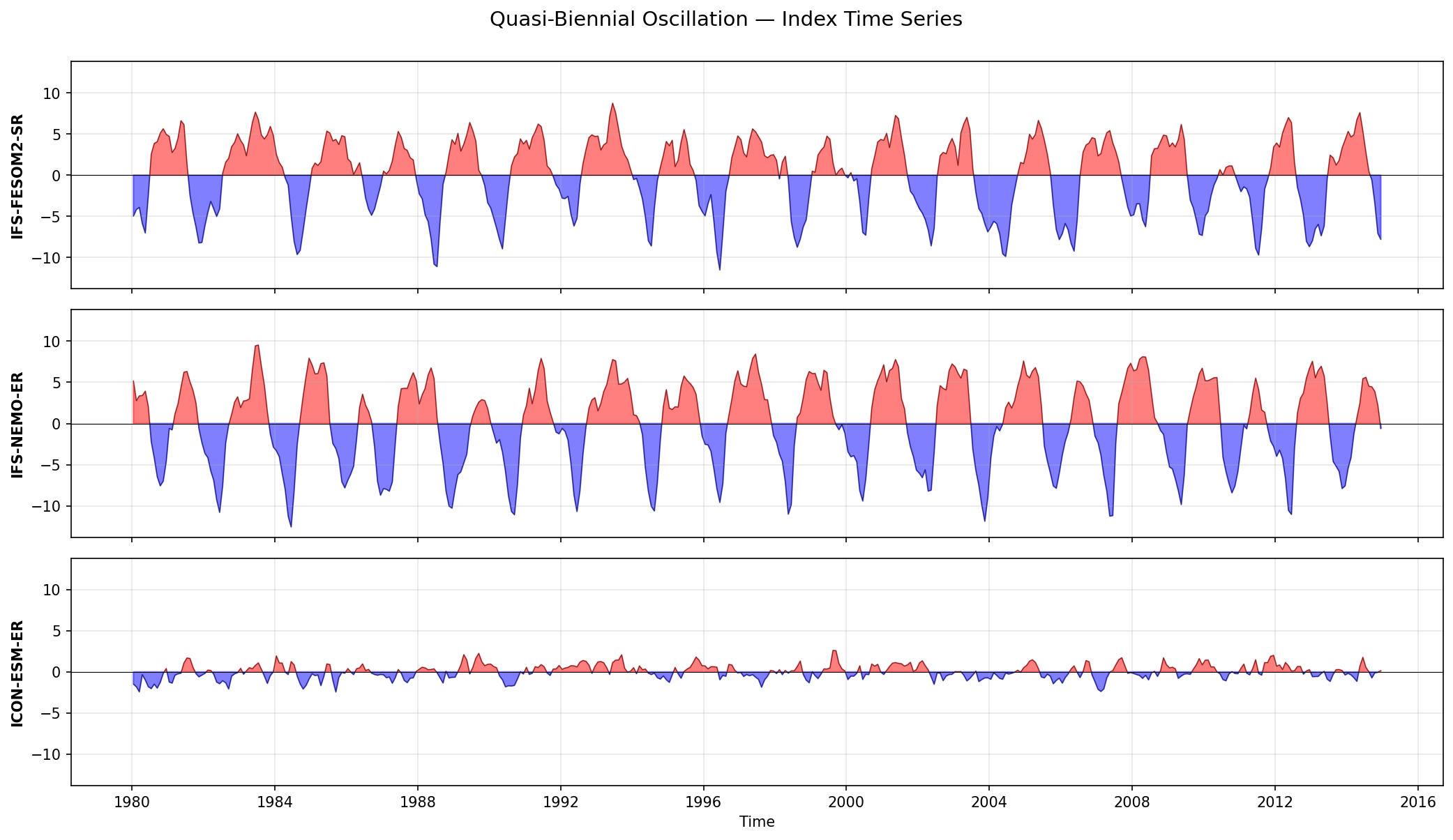
| Variables | ua |
|---|---|
| Models | IFS-FESOM2-SR, IFS-NEMO-ER, ICON-ESM-ER |
| Reference Dataset | ERA5 |
| Units | m/s |
| Period | 1980–2014 |
| IFS-FESOM2-SR | Std: 4.55 · Mean: -0.00 |
| IFS-NEMO-ER | Std: 5.30 · Mean: 0.00 |
| ICON-ESM-ER | Std: 0.88 · Mean: 0.00 |
Summary high
The IFS-based models (IFS-FESOM2-SR and IFS-NEMO-ER) successfully simulate a robust Quasi-Biennial Oscillation (QBO) with realistic periodicity and amplitude, whereas ICON-ESM-ER fails to generate a discernible QBO signal.
Key Findings
- IFS-NEMO-ER and IFS-FESOM2-SR exhibit clear, regular transitions between westerly (positive) and easterly (negative) phases with a periodicity characteristic of the QBO (approx. 2-3 years).
- ICON-ESM-ER shows no organized QBO variability, characterized by low-amplitude noise (standard deviation ~0.88 m/s) compared to the IFS models (standard deviations ~4.5–5.3 m/s).
- IFS-NEMO-ER produces a slightly stronger QBO amplitude (std: 5.30 m/s) than IFS-FESOM2-SR (std: 4.55 m/s), with peaks frequently exceeding magnitude 5 m/s.
Spatial Patterns
While this is a time series, the temporal pattern in the IFS models shows the expected 'flat-topped' westerlies and sharper easterly transitions typical of stratospheric zonal wind oscillations. ICON-ESM-ER displays no temporal structure, fluctuating near zero.
Model Agreement
There is a strong dichotomy: the two IFS configurations agree on the presence and approximate magnitude of the phenomenon, while ICON-ESM-ER is a distinct outlier that fails to capture stratospheric dynamics.
Physical Interpretation
The QBO is driven by wave-mean flow interactions involving upward propagating Kelvin, Rossby-gravity, and gravity waves. The success of the IFS models suggests they have sufficient vertical resolution in the stratosphere and/or effective non-orographic gravity wave drag parameterizations to support this oscillation. The failure of ICON-ESM-ER implies insufficient vertical resolution, inadequate gravity wave forcing, or excessive damping in the equatorial stratosphere.
Caveats
- The figure does not overlay the observational reference (ERA5), preventing assessment of phase synchronization or exact period length accuracy.
- The specific pressure level used for the index is not explicitly defined in the visual, though amplitudes suggest standard stratospheric levels (e.g., 30 or 50 hPa).
Southern Annular Mode — Spatial Pattern
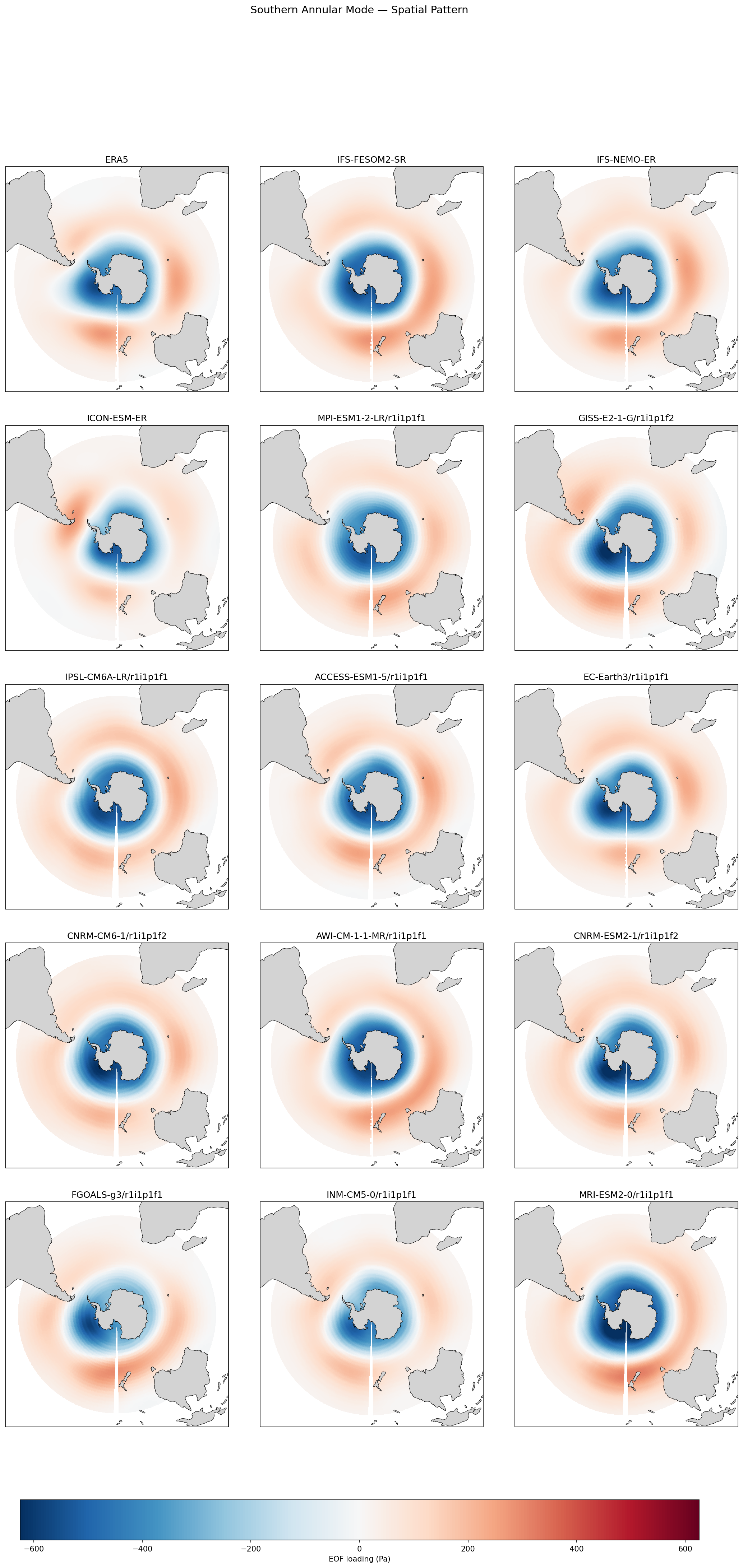
| Variables | psl |
|---|---|
| Models | IFS-FESOM2-SR, IFS-NEMO-ER, ICON-ESM-ER |
| Reference Dataset | ERA5 |
| Units | Pa |
| Period | 1980–2014 |
| IFS-FESOM2-SR | Variance Explained: 0.37 |
| IFS-NEMO-ER | Variance Explained: 0.30 |
| ICON-ESM-ER | Variance Explained: 0.25 |
| ERA5 | Variance Explained: 0.27 |
Summary high
This multi-panel figure evaluates the spatial pattern of the Southern Annular Mode (SAM) via the leading EOF of sea level pressure (PSL), comparing high-resolution EERIE simulations (IFS-FESOM2-SR, IFS-NEMO-ER, ICON-ESM-ER) and a suite of CMIP6 models against ERA5 reanalysis.
Key Findings
- All EERIE models successfully capture the classic annular structure of the SAM, featuring a negative pressure anomaly over Antarctica and a positive anomaly ring in the mid-latitudes, consistent with ERA5.
- IFS-FESOM2-SR overestimates the SAM's dominance, with the mode explaining 36.5% of total variance compared to 27.3% in ERA5, whereas IFS-NEMO-ER (29.9%) and ICON-ESM-ER (25.1%) are closer to the observational value.
- The spatial patterns in the high-resolution EERIE models are robust and compare favorably to the spread seen in the CMIP6 ensemble, where some models (e.g., FGOALS-g3, INM-CM5-0) show weaker gradients or less coherent structures.
- ICON-ESM-ER exhibits a slight zonal asymmetry near the Drake Passage/Antarctic Peninsula relative to ERA5, with positive loadings protruding further south.
Spatial Patterns
The dominant pattern is a zonally symmetric dipole with a node at approximately 60°S. ERA5 shows a central low (negative loading ~-400 to -600 Pa) over Antarctica surrounded by a mid-latitude high (positive loading ~200-400 Pa). This structure is well-reproduced across the EERIE models, though the precise location of the zero line and the amplitude of the mid-latitude lobes vary slightly.
Model Agreement
There is high inter-model agreement regarding the sign and general shape of the SAM pattern. The IFS variants (NEMO and FESOM) show particularly strong spatial correlation with ERA5. The CMIP6 ensemble generally supports the pattern but exhibits larger variance in amplitude and zonal symmetry.
Physical Interpretation
The SAM represents the north-south vacillation of the Southern Hemisphere eddy-driven jet stream and the associated redistribution of atmospheric mass. The faithful reproduction of this pattern implies that the models generally capture the mean location and variability of the SH storm tracks and the geostrophic balance governing the meridional pressure gradients.
Caveats
- The analysis relies on the leading EOF; higher-order modes (e.g., zonal waves) are not analyzed here but influence local variability.
- Variance explained percentages are sensitive to the domain and pre-processing, though relative differences (e.g., IFS-FESOM vs ERA5) are robust.
Southern Annular Mode — Seasonal Variance Profile
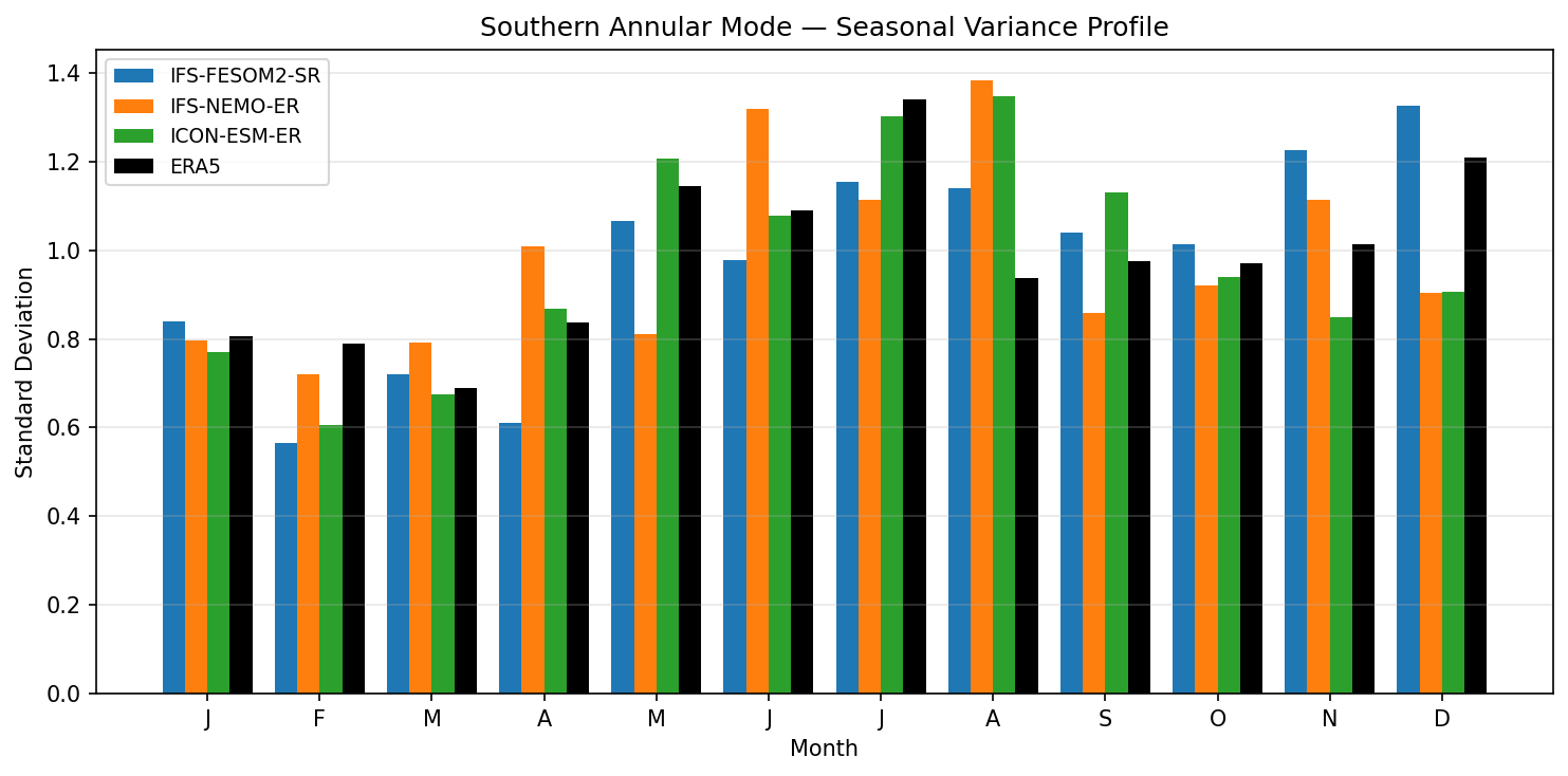
| Variables | psl |
|---|---|
| Models | IFS-FESOM2-SR, IFS-NEMO-ER, ICON-ESM-ER |
| Reference Dataset | ERA5 |
| Units | Pa |
| Period | 1980–2014 |
| IFS-FESOM2-SR | Peak Month: 12.00 · Peak Std: 1.33 · Annual Std: 1.00 |
| IFS-NEMO-ER | Peak Month: 8.00 · Peak Std: 1.38 · Annual Std: 1.00 |
| ICON-ESM-ER | Peak Month: 8.00 · Peak Std: 1.35 · Annual Std: 1.00 |
Summary high
This figure illustrates the seasonal cycle of the Southern Annular Mode (SAM) variability, showing the monthly standard deviation of the SAM index for three high-resolution models compared to ERA5.
Key Findings
- ERA5 displays a bi-modal peak in SAM variability, with maxima in austral winter (July) and summer (December), and a minimum in austral autumn (March).
- ICON-ESM-ER accurately reproduces the austral winter ramp-up (May-July) but erroneously sustains peak variability into August, where ERA5 shows a sharp decline.
- IFS-FESOM2-SR captures the austral summer (December) peak best, exceeding ERA5 slightly, but underestimates variability during the austral winter onset (May-June).
- IFS-NEMO-ER exhibits a noisy seasonal cycle with unrealistic spikes in April and August, failing to capture the smooth seasonal transitions seen in observations.
Spatial Patterns
While the diagnostic is temporal, it reflects the seasonal modulation of the Southern Hemisphere extratropical circulation. The observed pattern is characterized by enhanced variance during the active jet seasons (winter and summer) and suppressed variance during the equinoctial transition in autumn.
Model Agreement
Inter-model agreement is poor regarding the phase of maximum variability. ICON-ESM-ER and IFS-NEMO-ER bias towards a late-winter peak (August), while IFS-FESOM2-SR biases towards a summer peak (December). None of the models fully capture the specific double-peak structure of ERA5, though ICON performs best for the winter maximum and IFS-FESOM2 for the summer maximum.
Physical Interpretation
The SAM variability is driven by eddy-mean flow interactions in the Southern Hemisphere jet. The strong December peak in IFS-FESOM2-SR suggests a robust (possibly too strong) representation of stratosphere-troposphere coupling during the breakdown of the polar vortex. Conversely, the extended winter activity in ICON-ESM-ER and IFS-NEMO-ER (August overshoot) suggests biases in the persistence of the eddy-driven jet or delayed seasonal transition in the ocean-atmosphere coupling.
Caveats
- The indices are likely normalized based on the full annual cycle, so values >1 indicate months more variable than the annual average.
- Internal variability can be large for SAM seasonal statistics over a 35-year period; differences in peak timing might partly reflect sampling noise.
Southern Annular Mode — Power Spectrum
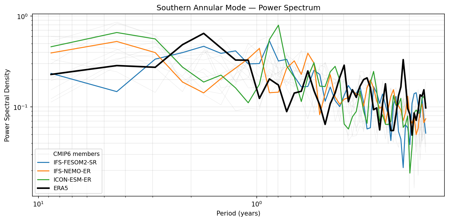
| Variables | psl |
|---|---|
| Models | IFS-FESOM2-SR, IFS-NEMO-ER, ICON-ESM-ER |
| Reference Dataset | ERA5 |
| Units | Pa |
| Period | 1980–2014 |
Summary medium
This figure displays the power spectral density of the Southern Annular Mode (SAM) index, comparing the frequency distribution of variability in three high-resolution coupled models against ERA5 reanalysis and the CMIP6 ensemble.
Key Findings
- ERA5 (black) exhibits a broad spectral peak in the interannual band (approximately 2–3 year periods).
- ICON-ESM-ER (green) shows anomalously high power at decadal scales (>5 years) and a sharp, distinct peak near the 1-year period which is not present in observations.
- IFS-FESOM2-SR (blue) most closely captures the spectral shape and magnitude of ERA5 in the critical 2–5 year interannual band.
- IFS-NEMO-ER (orange) overestimates variance at low frequencies (>5 years) while underestimating power in the 2–4 year band relative to ERA5.
Spatial Patterns
The spectra generally exhibit 'red noise' characteristics (higher power at longer periods). At frequencies higher than 1 year (right side), all models and ERA5 show similar power decay, consistent with internal atmospheric variability.
Model Agreement
IFS-FESOM2-SR agrees best with the observational reference (ERA5). Both IFS-NEMO-ER and ICON-ESM-ER diverge significantly at lower frequencies (decadal scales), showing higher variance than the specific ERA5 realization, though they remain within the broad spread of the CMIP6 ensemble (grey lines).
Physical Interpretation
The SAM is an internal atmospheric mode with a short intrinsic timescale (~10 days), but its spectrum is 'reddened' (enhanced low-frequency power) by coupling with the high-thermal-inertia Southern Ocean. The excessive low-frequency power in ICON-ESM-ER and IFS-NEMO-ER suggests potentially too strong ocean-atmosphere coupling feedbacks or model drift. The spike near 1 year in ICON-ESM-ER may indicate residual seasonality or a mode-locking artifact.
Caveats
- The analysis period (1980–2014, 35 years) is short relative to the decadal periods shown on the left, leading to large statistical uncertainty in the low-frequency spectral estimates.
- The CMIP6 spread is very large, indicating significant internal variability or structural uncertainty in representing SAM timescales across the generation of models.
Southern Annular Mode — Index Time Series
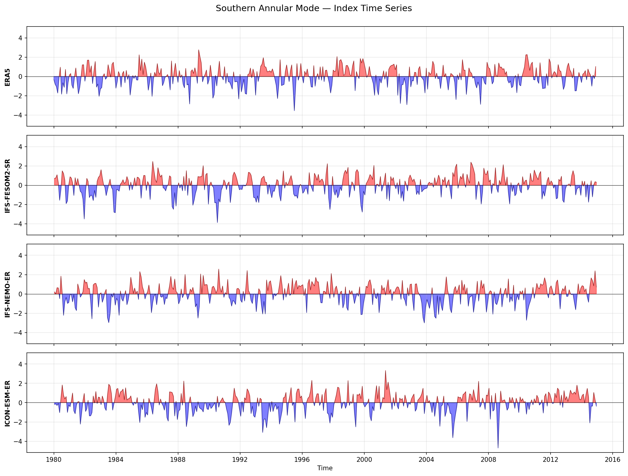
| Variables | psl |
|---|---|
| Models | IFS-FESOM2-SR, IFS-NEMO-ER, ICON-ESM-ER |
| Reference Dataset | ERA5 |
| Units | Pa |
| Period | 1980–2014 |
| IFS-FESOM2-SR | Std: 1.00 · Mean: 0.00 |
| IFS-NEMO-ER | Std: 1.00 · Mean: 0.00 |
| ICON-ESM-ER | Std: 1.00 · Mean: 0.00 |
Summary high
This figure compares the monthly time evolution of the standardized Southern Annular Mode (SAM) index from 1980 to 2014 across three high-resolution coupled models (IFS-FESOM2-SR, IFS-NEMO-ER, ICON-ESM-ER) and ERA5 reanalysis.
Key Findings
- All three models exhibit realistic high-frequency temporal variability in the SAM index, statistically resembling the stochastic character of the ERA5 reanalysis.
- The frequency and magnitude of extreme SAM phases (indices exceeding ±2 to ±3 standard deviations) are well-reproduced in the simulations, indicating a good representation of the tail of the dynamical distribution.
- No obvious pathological behaviors (e.g., unrealistic periodicity, drifts, or 'stuck' regimes) are visible in the model time series, suggesting stable simulation of Southern Hemisphere extratropical dynamics.
Spatial Patterns
N/A (Time series analysis). Temporally, the data shows characteristic 'red noise' behavior with significant month-to-month fluctuations superimposed on interannual variability.
Model Agreement
The models show high statistical agreement with ERA5 regarding the variance structure and intermittency of the SAM. Since these are free-running coupled simulations, the chronological phasing of specific peaks and troughs does not match observations, which is the expected behavior.
Physical Interpretation
The SAM describes the meridional vacillation of the Southern Hemisphere eddy-driven jet. The realistic variability implies that the models correctly capture the internal atmospheric dynamics (eddy-mean flow interactions) driving this mode. The ability of the models to generate similar excursion magnitudes suggests that the high resolution (~10 km) allows for appropriate synoptic-scale eddy activity feeding into the low-frequency mode.
Caveats
- The indices are standardized (mean ~ 0, std = 1), which facilitates variability comparison but masks any potential biases in the absolute amplitude (Pa) or spatial structure of the SAM pattern.
- The dense monthly plotting without a trend line or low-pass filter makes it difficult to visually evaluate whether the models capture the historical positive trend in the SAM associated with ozone depletion and greenhouse gas forcing.